Theory of Characteristic Modes

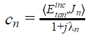
Characteristic modes or characteristic currents can be represented quantitatively as eigenfunctions of the following generalized eigenvalue problem:

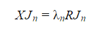
where

λ_n = eigenvalue

J_n= eigenvector

R and X are the real and imaginary parts of the impedance operator.

The total power exiting a surface is:

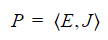
Where E is the electric field on the surface and J is the surface current. We can use the electric field integral equation to relate these two quantities to obtain

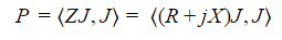
Where R and X are the real and imaginary parts of the EFIE impedance matrix, Z = R + jX. The real part of P is the power radiated and the imaginary part is the power stored in the near field. For antenna design, we want to maximize the power radiated, or equivalently, minimize the power stored in the near field. The solution to this minimization problem is the generalized eigenvalue problem given above.

Qualitatively, characteristic modes are equiphase current modes, which can be computed for metallic and dielectric structures of arbitrary shapes and sizes and are independent of any excitation. Characteristic modes not only allow modal analyses of conductors but they are also useful for antenna design and placement, and the properties of the characteristic modes provide insight and valuable information for designing antennas. In fact, these quantities provide a physical interpretation of the radiating characteristics of an antenna. Therefore, understanding them can be very useful in problems involving syntheses, analyses, and optimization of antennas and scatterers. These quantities, known as characteristic value and characteristic current, are obtained by solving the above generalized eigenvalue problem. Together they define a characteristic mode. In addition to characteristic value and characteristic current, HFSS also depicts these quantities in the form of characteristic angle and modal significance to provide a practical insight into the behavior of the modes.

Using the standard Galerkin discretization of the EFIE, the characteristic values and characteristic currents in a lossless system are purely real. When the characteristic value is 0, no power is stored in the near field--all the power is radiated. From the characteristic value, you can make the following inferences:

• when λ_n = 0, the mode is externally resonant.
• when λ_n > 0, the mode is inductive (the energy is stored in a magnetic field).
• when λ_n < 0, the mode is capacitive (the energy is stored in an electric field).

Since the characteristic values can range from -infinity to +infinity, it’s more convenient to represent this quantity in terms of characteristic angle.

Characteristic Angle

Characteristic angle represents the phase lag between the electric field and surface current on a conductor. Mathematically, characteristic angle is defined as:

α_n=180°- tan^-1λ_n

Characteristic Angle can range from 90 deg to 270 deg leading to the following possibilities:

• when α_n= 180 deg, the mode is externally resonant.
• when 90 deg < α_n < 180 deg, the mode is inductive.

• when 180 deg < α_n < 270 deg, the mode is capacitive.

Modal Significance

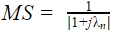
Modal Significance, as the term indicates is a measure of how significant a mode is for solving the EFIE at a given frequency. It also determines how hard or how easy it is to excite a mode. Mathematically, Modal Significance is defined as:

Since the characteristic current diagonalizes both the real and imaginary parts of the impedance matrix, we can define

ν_n=1+ jλ_n

which is an eigenvalue of the EFIE impedance matrix, Z = R+ jX. The eigenvalue is significant since its magnitude provides information about how well the corresponding mode radiates. Using the impedance matrix, eigenvalues, as well as the characteristic currents, the EFIE is analytically solved and the modal excitation coefficients are obtained as follows--

Thus, we write that the magnitude of the coefficient must be

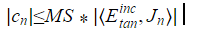
where MS is the modal significance. The maximum value of modal significance is 1. This happens when the mode is externally resonant. Modal significance can decay to zero when the mode is not resonant.

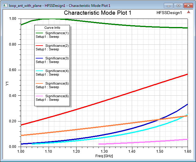
Depending upon the electrical size of the antenna, when you perform a characteristic mode analysis, a large number of modes can be computed. From a practical standpoint, when an object is not electrically large, most of the modes are difficult to excite since their characteristic values are far from 0. While one can generate plots of the characteristic value (λ_n) as a function of frequency, it’s often more convenient to plot a quantity like Modal Significance as a function of frequency. This is because one is interested mostly in the characteristic values close to 0, in other words, MS =1 where the mode is externally resonant. A graph depicting modal significance as a function of frequency can be very useful because such a graph lets you easily examine the importance of the modes and understand which of the modes contribute significantly to the radiated power (MS = 1), and the ones that are decaying (MS = 0).

Characteristic mode analyses give physical insight of the current pattern that can exist on an antenna and the platform upon which it operates. This insight can be valuable to a design engineer and help as a first step toward achieving correct antenna placement on electrically medium-sized structures.

The following designs are practical applications of characteristic mode analysis in HFSS.

Loop Antenna of a Cell Phone Chassis

The following figure shows a cell phone chassis, which contains a simple plate representing its backplane. It also has a loop antenna.

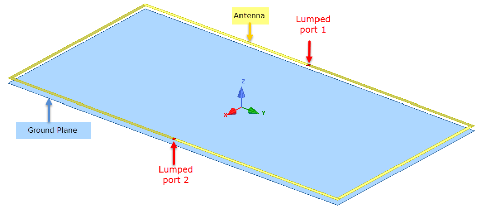
The boundary conditions are shown below. The plate and the antenna are assigned Perfect E boundaries. Also, the antenna modes are excited by assigning lumped ports. The simple plate acts as the antenna’s ground plane, and its shape and size affect the performance of the antenna significantly. Therefore, if you perform a characteristic modal analysis of this design in HFSS, you can obtain critical information about the current modes and their pattern for this structure. Characteristic Mode Analysis solution type is chosen for this design. The design is analyzed at solution frequency of 1.6 GHz. Minimum Modal Significance is 0.02 so all modes above this threshold are calculated by HFSS. On the Edit Sources panel, you can configure the type of CMA Excitations as Port or Modes.

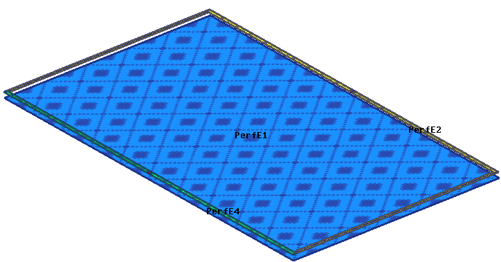
Settings in the Edit Sources panel can help you understand the impact of the CMA excitations on the behavior of modes and their current patterns.

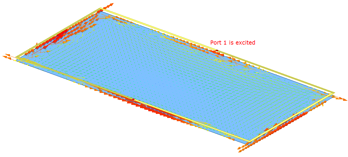
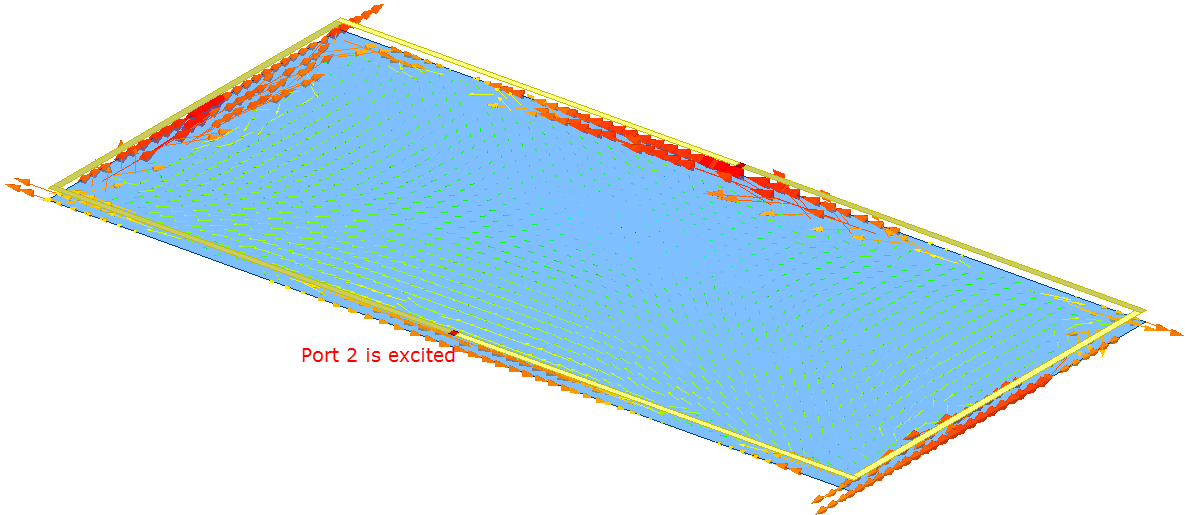
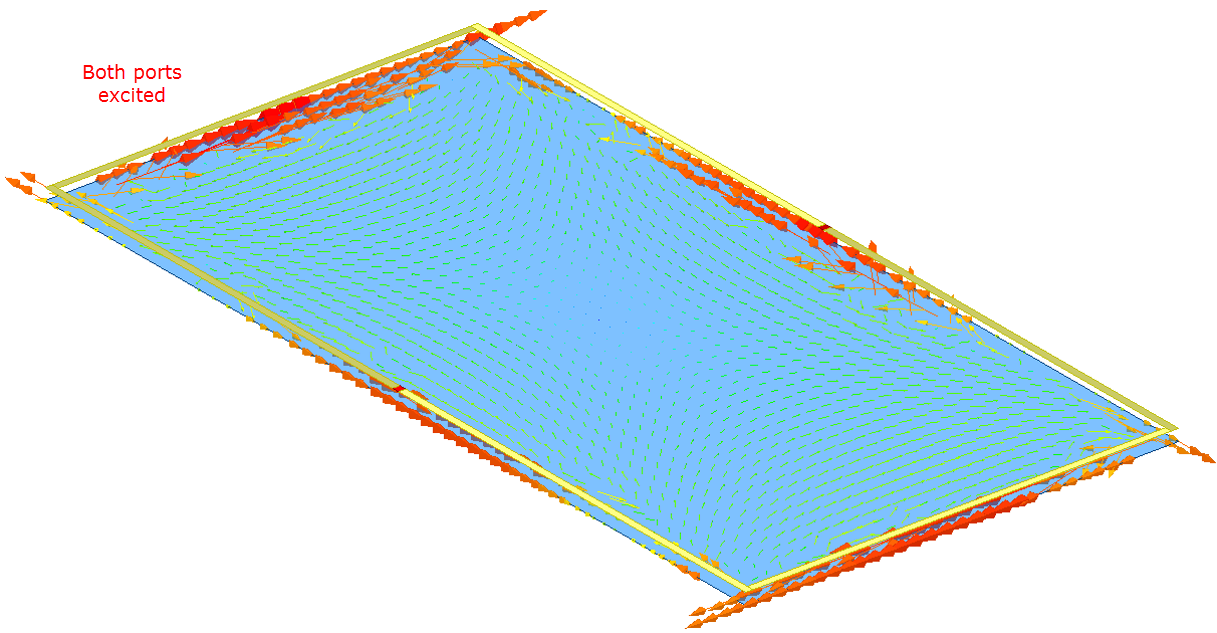
To illustrate, you can plot the characteristic currents in this design and understand how the mode behavior is affected by the port excitations. Depending upon how you define the CMA Port excitations, different modes are excited accordingly on the plane. For example, if you define lumped port 1 as the excitation for this structure, the current pattern mostly consist of mode 3. However, the other modes do have some contribution to the field pattern. Similarly, when lumped port 2 is excited the current pattern mostly consists of mode 3. If both ports are excited the pattern is identical to mode 3.

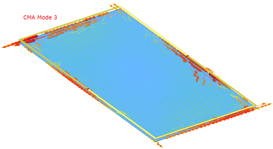
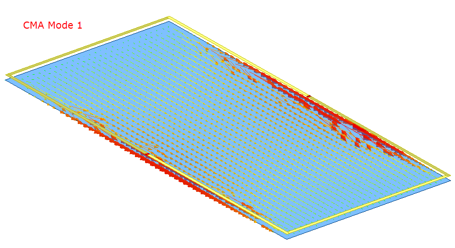
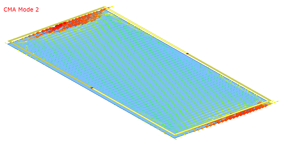
The above images illustrate the mode currents when the CMA Excitations are configured to be modes 1, 2, or 3. Mode 3 is the dominant mode. Characteristic angles associated with the current modes can be plotted as a function of frequency.

Once you have completed the modal analysis of your design, you can make modifications to your design as needed to excite the desired modes. This characteristic mode analysis example demonstrates how by viewing the current patterns you can excite only those modes of interest and maximize radiated power. Design modifications depending upon the modes you want to excite can improve antenna performance.