Obtaining Broadband Matching between Huray and Hammerstad Models

This topic contains the procedure for obtaining broadband matching between Huray and Hammerstad models.

The simplest way to create a Hammerstad model that is in some sense close to a Huray model is to ensure the maximum values of the models are the same.

Then, try to line up the models at their 50% crossing points. For the Hammerstad model, that occurs when (1):

For the Huray model, the 50% point is reached when (2):

By solving for f, the equation reduces to the following (3):

Therefore, for 50% of points to agree, the following condition must be realized (4):

Using equation 4 and relating back to the model parameters, the following is obtained (5):

Compare the two models. For the Hammerstad model, set SF=3 and Δ=1.766m and let the material be copper. This conveniently yields f_HJ = 1 GHz.

Using the preceding relations, the corresponding Huray model has SR=4/3 and a=2.854μm.

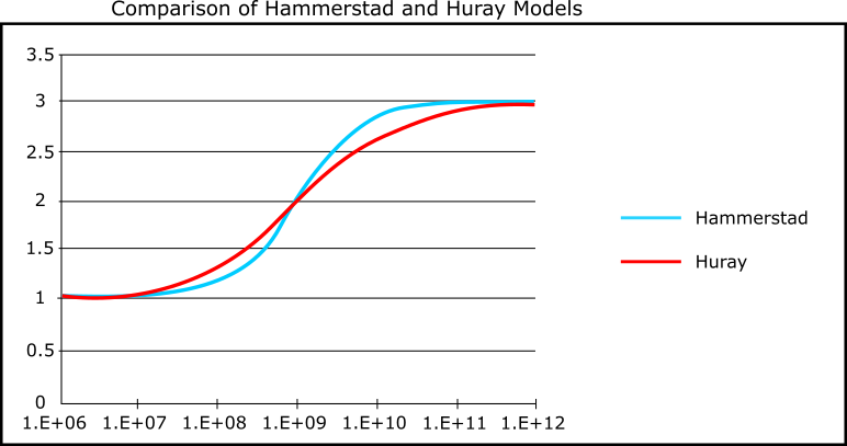
Plots of H_HJ(f) and H_HH(f) are shown in the following figure.

The figure demonstrates the expected match between the two curves at the 50% point (1 GHz), and the expected match at the low and high frequency extremes. It is also clear the Hammerstad model transitions between low and high frequency more rapidly than the Huray model. This is inherent to the mathematical functions used in the model. Since the Huray model is based on the physics of the underlying loss mechanism while the Hammerstad model is a curve fit, it is reasonable to expect the Huray model to be more realistic.

The preceding model-matching procedure potentially may be critiqued as follows:

• The matching is exact at some (three) points and is decent across the entire frequency range.
• The computed snowball radius is actually greater than the RMS surface roughness value. This does not seem realistic.

An alternative procedure is to try matching the two models at low frequencies. The rationale for doing this is the loss measurements used to derive a Hammerstad model are likely to be taken mainly at frequencies well beneath the 50% point. Therefore, the higher frequency values might not be given as much weight in the matching process. This approach is described below.

Obtaining Better Low Frequency Matching

The low frequency match could be improved by shifting the Huray model curve to the right. Such a shift can be accomplished by reducing the value of the snowball radius; this increases the Huray corner frequency f_HH.

No unique method exists to do this since there are many different frequency ranges and error metrics that could be used. Results obtained from some trial and error experiments reveal that a good starting point is using the broadband parameter values:

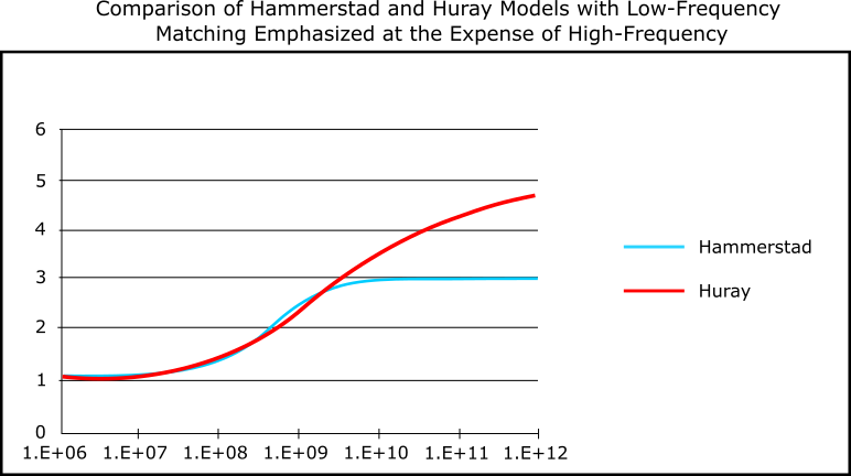
A match qualitatively similar to that shown in the following figure is obtained by choosing:

For more information, see references below.

Setting a = 1.148μm and SR = 2.667 results in the following comparison:

The match between the two is very good up to about 4 GHz, well beyond the 50% crossing point of the Hammerstad model at 1 GHz. Beyond this frequency, the fitted Huray model predicts significantly higher losses (66% greater) than the Hammerstad model. This is the price paid for the improved low frequency match. Of course it was assumed the Hammerstad model may not be accurate in this higher frequency range anyway.

To summarize, the Hammerstad model is fundamentally different from the Huray model. Since Hammerstad is strictly a mathematical model and the Huray model is a physics-based model, the conversion between the two is not exact. An approximate conversion is indeed possible, as shown, and the choice of conversion process depends on whether a broadband or a low-pass match is chosen. Two conversion schemes have been described here, but a continuum of different choices is available.

Expect that any usable conversion scheme has Huray model parameters that satisfy the following bounds:

and

References:

1. E. Bogatin, D. DeGroot, P.G. Huray, and Y. Shlepnev. "Which one is better? Comparing options to describe frequency dependent losses." DesignCon, 2013.