Distributed Analysis Configuration - Job Distribution Tab
On the Analysis Configuration window, the Job Distribution tab allows you to manually enable specific types of job distribution and enable multi-level solves.
The Job Distribution tab is disabled if you selected Use Automatic Settings.
Different design types have different job distribution types.

The job distribution list allows you to specify which job distribution types
to allow for the current analysis configuration. Use
the check boxes enable and disable distribution types. At solve time,
Enabling a distribution type does not mean it will be used. It must be also allowed by the solve setup. If you enable a distribution type for a given setup, and distribution is allowed, the preview window updates to describe the distributions. Note that enabled distribution types apply to all setups of the given design type, so it is possible for different setups in a design to be solved using different distribution types.
The concurrent initial mesh generation workflow with Distributed Mesh Assembly relies on the MPI based distribution technology inside the MeshAssemblyManager. The decision whether to launch sequential or parallel mesh generation is based on the combination of the number of individual meshes present, the HPC setting, and the number of tasks available.
- If there’s only one single mesh or if curvilinear contact exists: then normal initial mesh workflow with single G3dmesher will be launched.
- If there are more than one individual mesh and no curvilinear contact exists:
- If Use Automatic Setting is not selected, under the Job Distribution tab, if “Mesh Assembly” is not enabled, then meshes will be generated sequentially. If “Mesh Assembly” is enabled and user assigns more than 1 tasks, then parallel mesh generation will be launched.
- If Use Automatic Setting is selected and user assigns more than 1 core, then parallel mesh generation will be launched.
- If Use Automatic Setting, the number of MPI tasks will be the number of cores user assigned or the number of geometries to be meshed, whichever is smaller. If there are more geometries than cores, the geometries will be dynamically assigned to tasks. If there are more cores than geometries, the remaining available cores will provide some of the tasks with multi-thread capabilities.
All the detailed progress information from the Mesher is suppressed and the progress will report the number of meshes being finished. All the mesh profiles will be available under profile report and the mesh feedback will also be available under mesh feedback tool.
Enabled distribution types are listed when you select a configuration in the HPC and Analysis Options window.

When you run a simulation, the Messages window describes distributions.

When you view the Solution Profile, distributions for unitCell show as parallel Volume Tasks.

Distribution Levels
For products and designs that support two-level distribution, you can select either single or two-level distribution.
If you select single level, one distribution type will be applied at each stage of the solution process. If multiple types are available, the higher-level solution will generally be distributed. All machine tasks will be used by the single-level distribution.
Single-level Distributions
In a single-level distribution, one distribution type is applied at each stage of the solution process. Common stages include LastAdaptive, Sweep, and Parametric. All machine tasks will be used by the single-level distribution.

Supported distribution types include:
- Optimetrics Variations
- Frequencies
- Mesh Assembly
- Transient Excitations
- Domain Solver(for Technical details, see Domain Decomposition Method)
- Iterative Solver Excitations(for Technical details, see Multiprocessing and the Iterative Solver)
- Direct Solver Memory(for Technical details, see Distributed Memory Solutions with HFSS)
Solver distributions require MPI. See: Setting HPC and Analysis Options.
Parallel distribution types (such as Optimetrics Variations,
Frequencies
Memory distribution types (such as
When multiple distribution types are available, the higher-level solution will generally be distributed. For example, when both Optimetrics Variations and Iterative Solver Excitations are enabled, Optimetrics Variations will be distributed. When both Optimetrics and Mesh Assembly, are selected Optimetrics are distributed. Domain Solver and Direct Solver Memory are exceptions because they are required; even though they are lower level, these types are distributed instead of parallel distribution types.
Two-level Distributions
Selecting Enable two-level enables the Distributed solutions at first level box.
In a two-level distribution, the first level distributes the specified number of solutions. Each solution will then use a subset of machine tasks to distribute the second level. A solver distribution type must be available for the second level; otherwise, single-level distribution will be applied.
For two-level distribution, the total number of tasks must be greater than or equal to the number of tasks for level 1.

The following
- A parametric setup distributing Optimetrics variations as level 1 and iterative solver excitations as level 2.
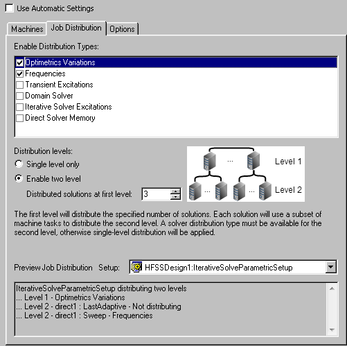
- A parametric setup for a non-transient problem distributing optimetrics variations as level one and frequencies as level 2.
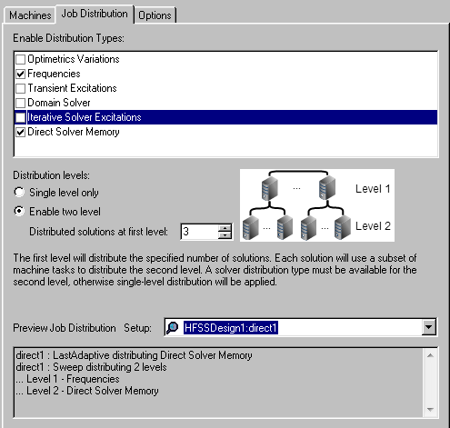
- A frequency sweep distributing frequencies as level 1 and direct solver memory as level 2.
- A parametric setup for a transient network problem distributing optimetrics variations as level one and transient excitations as level 2.
The Analysis Configuration window displays a preview of the job distribution, if allowed for that configuration:

Here is another example:

For more information, see: Two-Level Distribution Guidelines.
HFSS Frequency Distribution
HFSS Frequency Distribution can be treated as both of first and second level distribution. The following bullets described the cases for an HFSS design with frequencies sweep setup and parametric solve setup (for non transient solution).
- In the Analysis Configuration window, if you select “Optimetrics Variations” and “Frequencies” with two-level distribution enabled, HFSS does two level distribution: first level, “Optimetrics Variations”; second level “Frequencies”. We can see this described in the “Preview Job Distribution” area:
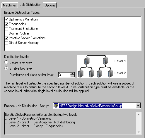
- In the Analysis Configuration window, if you select “Optimetrics Variations”, “Frequencies”, and “Iterative Solver Excitations“ with two-level distribution enabled, HFSS does two level distribution: first level, “Optimetrics Variations”; second level “Frequencies”. There is no “Iterative Solver Excitations“ distribution. We can see this in the “Preview Job Distribution” area:
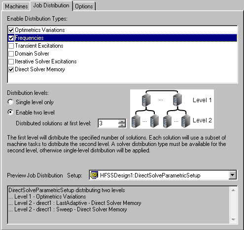
- In the Analysis Configuration window, if you select “Optimetrics Variations”, “Frequencies”, and “Direct Solver Memory“ (or “Domain Solver”) with two-level distribution enabled, and if “Direct Solver Memory“ option is selected in the solve setup, HFSS does two level distribution: first level, “Optimetrics Variations”; second level, “Direct Solver Memory“ (or “Domain Solver”). There is no “Frequencies” distribution. We can see this in the “Preview Job Distribution” area:
- In the Analysis Configuration dialog box, if you select “Frequencies”, and “Iterative Solver Excitations“( or “Direct Solver Memory“, or “Domain Solver”) with two-level distribution enabled and if you select “Direct Solver Memory“ option (or corresponding solver option) in the solve setup, HFSS only does two level distribution: first level, “Frequencies”; second level, “Iterative Solver Excitations“ (or corresponding solver. We can see this in the “Preview Job Distribution” area. See the following two examples. The first shows Enable Job Distribution Types for “Frequencies” and “Direct Solver Memory”.