Varying the Port Excitation

You can vary the voltage applied to a model by scaling its magnitude and modifying its phase in the Edge Port Definition window. A schematic of an excitation is shown in the following diagram. The voltage source model is in series with an impedance called Calibration Zo that is equal to the characteristic impedance of the port. Hence, renormalizing the port impedance change the port excitation model.

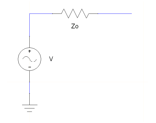
Zo is equivalent to the Full Port Impedance of the port. It is user-defined with the format "<real_part> + <complex_part>*i ohm" (e.g., example 50ohm + (-5ohm) * 1i). You can assign a variable as these values, (e.g., " resistance + (reactance) * 1i"). This variable can be dependent on the frequency, which allows use of a dataset for frequency dependent impedance, (e.g., pwl(ds1,freq) + (pwl(ds2,freq)) * 1i). The real part must be positive and the complex part non-zero if the resistance is zero. See lumped port theory for details.

To vary the applied voltage at a port:

1. Double-click the edge port in the project tree to open the Edge Port Definition window.

   

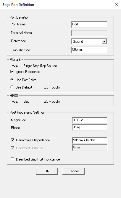
2. For the ignore reference option:

• If not selected, the port and the reference plane are physically connected. For most cases, this has better high frequency performance.
• If selected, the port and the reference plane are not connected. This is typically the better option for a stripline environment since a vertical current between two infinite ground planes can excite a parallel plate mode.

3. For the port solver option:

• If selected, the Z₀ and gamma are calculated and the port is calibrated.
• If not selected, Z₀ is user-defined (default is 50) and the port is not calibrated.

4. From the Magnitude field, enter the magnitude of the voltage applied at the port.

In general, you may use the default value of 1 volt. This specifies the solution's current is scaled so that the excitation source is 1 volt. To view the solution at a different excitation level, enter a different positive value for Magnitude. Only modes with non-zero magnitudes are used in post-processing.

5. From the Phase field, enter a phase of the voltage applied at the port.
6. Click OK.