Creating a Transient EMI Receiver Probe Report

The FFT-based (i.e., Fast Fourier Transform) virtual EMI receiver (i.e., Time Domain Scan) probe reduces EMI/EMC compliance test time.

Adding EMI Receiver Probes to the Design

Complete the following steps to add one or more EMI receiver probes to a circuit design.

1. If necessary, open the Component Libraries window by navigating to View. A check appears adjacent to Component Libraries if the window is open.
   

2. From the Component Libraries window, scroll to and expand Nexxim Circuit Elements > Probes.
   

3. Hold+click EMI_RCVR: EMI Receiver to select the probe and attach it to the cursor. Then drag the probe to an appropriate place in the Schematic Editor.
   

4. Click to drop the component at the chosen location.
   

5. To add multiple EMI receiver probes, repeat steps 4-5, as necessary.

6. If the user has not already done so, perform a Transient Analysis Simulation before continuing. (Refer to Circuit Transient Analysis ).

Creating a Transient EMI Receiver Plot

Complete the following steps to create a new transient EMI receiver plot report.

1. From the Project Manager window, expand Project Tree > [active design folder]. Then right-click Results and select Create Standard Report > Rectangular Plot to open the Report window.
   
   

2. From the Context group box, select EMI Receiver from the Domain drop-down menu.
   
   Choosing EMI Receiver reveals several new options beneath the Domain drop-down menu.
   

3. From the Net drop-down menu, select the net or port to which the appropriate EMI receiver component is connected  (e.g., net_47). Selecting the net or port simultaneously changes the selections in the Trace tab > Quantity list.
   
   

   Note: EMI Receiver Probe reports are generated from the available transient signals recorded during transient analysis. To ensure that an EMI receiver probe is connected to a signal recorded for post-processing, repeat step 1 to open the Report window. Ensure Transient is selected in the Solution drop-down menu, and Time in the Domain drop-down menu (i.e., the default selections). The Quantity list will populate with all of the signals available for post-processing reports.
   

4. The Start and Stop fields allow the user to select specific time frames within the transient analysis for EMI receiver analysis. Enter the desired values in the Start and Stop fields.
   

   Note: The Start/Stop values should fall within the range entered in the Step/Stop fields during Transient Analysis setup.
   

5. Gaussian window is the default window type as required in CISPR16-1-1 standard. If necessary, enter a different value between 50 - 97 in the Overlap Rate (%) field (default is 95). The window overlap rate determines the time step of EMI analysis. A higher percentage will result in a smaller time step, at the cost of more computation and increased simulation time.

6. The field Emission has options Radiated Emission (RE) and Conducted Emission (CE) to choose from. The Emission information doesn’t alter simulation settings or results, but shows up in plot name and title as part of a plot ID.

7. Select the appropriate band from the Band drop-down menu. Other than Band A, B, C/D and E as defined in CISPR16-1-1, CE or RE bands required for CISPR25 EMI/EMC analysis are included in the menu. Selecting a band simultaneously populates the RBW field and the selections in the Trace tab>Quantity list, based on those defined in CISPR16-1-1.
   

   Note:
   1. For a sub-band of a CISPR16 Band, the RBW of the CISPR16 Band is applied to the sub-band. For example, Band 30M-200MHz is a sub-band of CISPR16 Band C/D(30M-1GHz), RBW=120KHz of Band C/D is applied to the sub-band 30M-1GHz.
   
   2. Considering Band 150k-108MHz crosses two CISPR16 Bands, RBW=9KHz for Band B(150K-30MHz) and RBW=120KHz for Band C/D (30M-1GHz) are applied in analysis.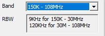
   
   3. For bands above 1GHz, RBW =1MHz is applied following standards CISPR16-1-1 and MIL-STD-461.

8. Ensure EMI Receiver is selected from the Category list (selected by Default).

9. From the Quantity list, select one or more detector options (i.e., Average, Peak, QuasiPeak, and/or RMS). It should be noted that for Bands above 1GHz, QuasiPeak detection is not supported.

   Note: Select multiple options from the Quantity list by Ctrl+clicking them.
   

10. From the Function list, select dBm or dBu, typically, depending on signal strength (<none> is selected by default).
    

11. Click New Report to create the new Transient EMI Receiver Plot N.
    

    Note: Band selection, signal length, and window Overlap Rate are directly related to the computation time and memory complexity of EMI analysis. When the required memory exceeds the available memory, post processing could terminate with an error message. Please follow the directions in the message and try again with lower overlap rate and/or shorter signal length.
    
    
    

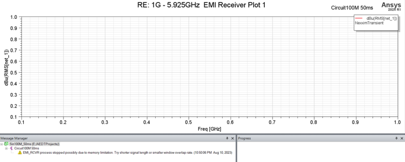
12. To close the Report window, click Close. If necessary, return to the Report window (i.e., from the Project Manager window, expand Results. Then right-click the appropriate report and select Modify Report...). Make changes to the selections in the Report window and click Add Trace to update the plot.
    
    
    

    Note: After modifying the selections in the Quantity list, the Function list will revert to its default selection (i.e., <none>).
    
    

Selecting Log/Linear From the Properties Window

From the report's Properties window, users can change many settings. For example, complete the following steps to change Axis Scaling from Linear to Log.

1. Double-click anywhere within the Schematic Editor to open the report's Properties window.
   

2. Navigate to the X Scaling tab.
   

3. From the Axis Scaling row, select Log from the Value drop-down menu (e.g., where Linear is currently).
   

4. Click Apply to save the new parameters.

5. Click OK to close the Properties window.

Selecting a New Minimum/Maximum From the Properties Window

Complete the following steps to modify the report's minimum/maximum resolution.

1. Double-click anywhere within the Schematic Editor to open the report's Properties window.
   

2. Navigate to the X Scaling tab.
   

3. Enter a new value in either the Min field, Max field, or both. Then check the corresponding boxes in the Specify Min/Specify Max fields.
   

4. Click Apply to save the new parameters.

5. Click OK to close the Properties window.