


Element Formulation
The cable element is formulated by adjusting the stiffness of a beam element based on the Timoshenko beam theory. For further details on the beam element in the Motion application, refer to the 2-Node Beam Element (Beam2) section in the Motion Theory Reference.
Stiffness Scale Factor
The stiffness of a cable element with a scale factor applied is as follows:
 | (14–1) |
where:
| α = bar scale factor |
| β = bending scale factor |
| γ = torsional scale factor |
| Kij = stiffness term of the beam element |
For a more detailed explanation of how each stiffness coefficient is calculated, refer to Equations 5.143 to 5.150 in the Beam Group section in the Motion Theory Reference.
The stress tensor of the cable element is calculated as follows:
 | (14–2) |
where:
 = stress tensor induced by axial load = stress tensor induced by axial load |
 = stress tensor induced by bending loads = stress tensor induced by bending loads |
 = stress tensor induced by torsion = stress tensor induced by torsion |
Note: It is important to note that while scale factors are applied to the stiffness matrix of the cable element for the purpose of constructing a practical equivalent model, the physical interpretation of the resulting stress tensor should be considered with caution. The stress calculation assumes linear scaling of axial, bending, and torsional components, which may not fully capture the complex behavior of real cable elements under load. This approach is primarily intended for approximation and reference. For cases where higher accuracy is required, it is recommended to first perform an initial analysis using the cable element and then use the resulting forces from this analysis for a subsequent, more detailed study with solid elements and non-linear material properties.
Geometry Representation
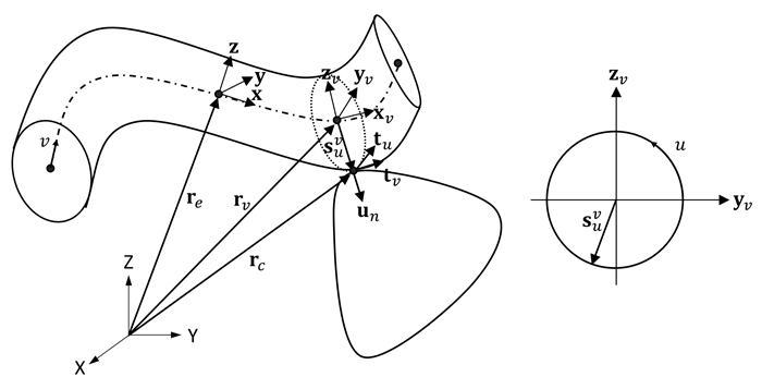
The geometry of the cable is represented based on the shape functions of the beam.
The position rv of a point on the neutral line of the cable element, along the axial direction with the natural coordinate v, is calculated as:
 | (14–3) |
where:
 = natural coordinate along the axial direction of the
cable = natural coordinate along the axial direction of the
cable |
 = orientation of the beam reference frame = orientation of the beam reference frame |
 = translational shape functions of the beam = translational shape functions of the beam |
 = generalized coordinates of the beam nodes with respect to the
element reference frame = generalized coordinates of the beam nodes with respect to the
element reference frame |
The position rc of a point on the surface of the cable element is defined by the natural coordinate u moving along a circle of radius R in a plane with the tangent vector at rv as the normal vector. This position is calculated as:
 | (14–4) |
where:
 = orientation of the reference frame at
v = orientation of the reference frame at
v |
 = Relative position between rc and rv, calculated as: = Relative position between rc and rv, calculated as: |
 | (14–5) |
where:
| R = beam cross-section radius |
The reference frame at an arbitrary
v is calculated as follows:
 | (14–6) |
 | (14–7) |
 | (14–8) |
 | (14–9) |
 | (14–10) |
where:
 = differentiated shape functions of the beam = differentiated shape functions of the beam |
 = user-defined direction vector = user-defined direction vector |
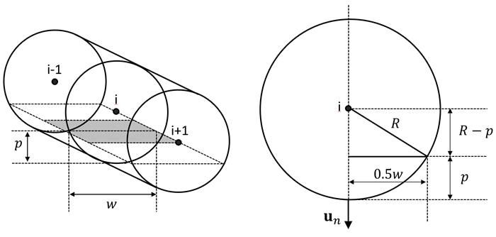
Contact Area
The contact area of the cable is assumed to be rectangular. The contact area for the i-th node is:
 | (14–11) |
where:
 = the length of the jth element
containing the ith node = the length of the jth element
containing the ith node |
w is calculated using the Pythagorean theorem as:
 | (14–12) |
where:
| p = contact penetration |
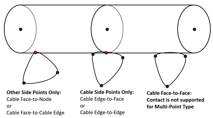
Finding the Exact Contact Point for a Cable
- Multi-Point Surface Type
When the Surface type is set to , the contact detection rules for cables follow the general contact rules, but the application of equations to find the exact contact point differs. In cable elements, the beam node itself does not come into direct contact. Instead, the cable's cross-sectional circle, where the beam node is located, is treated as an edge to determine the exact contact point.
Table 14.2: Method for finding contact points for Multi-Point type
Multi-Point Cable Edge to Face Cable Edge to Edge Cable Face to Node or Cable Edge Both O O O Cable Side Points Only O O X Other Side Points Only X X O
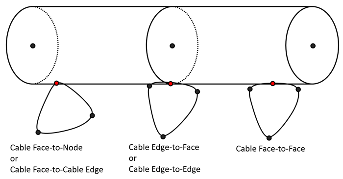
- Behavior for Surface Type
When the Surface type is set to , the standard contact rules apply. However, the nodes do not make direct contact, and instead, the cable's cross-sectional circle, where the beam node is located, is treated as an edge to determine the exact contact point. For a more detailed explanation of how to determine the exact contact point, refer to the Method for Finding Exact Contact Point Position section in the Motion Theory Reference.
Note:
If the cable element is sufficiently small compared to the opposing contact surface, or if the curvature of the opposing surface is not large, you should set the Surface Type to in the Contact properties and set the Point Check to .
If the contact involves smaller structures than the cable element or requires cable face-to-face contact, you should set the Surface Type to in the Contact properties.