


In the Ansys CFD codes the following SRS models are available:
Scale-Adaptive Simulation (SAS) models
SAS-SST model (Fluent, CFX)
Detached Eddy Simulation (DES) models
DES-SA (DDES) model (Fluent)
DES-SST model (Fluent (also DDES), CFX)
Realizable
 DES model (Fluent)
Shielded Detached Eddy Simulation (SDES)
All
 -equation based 2-equation models in
Fluent.
-equation based 2-equation models in
Fluent.Stress-Blended Eddy Simulation (SBES)
All
 -equation based 2-equation models in Fluent and
CFX.
-equation based 2-equation models in Fluent and
CFX.Large Eddy Simulation (LES)
Smagorinsky-Lilly model (+dynamic) (Fluent, CFX)
WALE model (Fluent, CFX)
Kinetic energy subgrid model dynamic (Fluent)
Algebraic Wall Modeled LES (WMLES) (Fluent, CFX)
Embedded LES (ELES) mode
Combination of all RANS models with all non-dynamic LES models (Fluent)
Zonal forcing model (CFX)
Synthetic turbulence generator
Vortex method (Fluent)
Harmonic Turbulence Generator (HTG) (CFX)
In principle, all RANS models can be solved in unsteady mode (URANS). Experience
shows, however, that classical URANS models do not provide any spectral content,
even if the grid and time step resolution are sufficient for that purpose. It has
long been argued that this behavior is a natural outcome of the RANS averaging
procedure (typically time averaging), which eliminates all turbulence content from
the velocity field. By that argument, it has been concluded that URANS can work only
in situations of a "separation of scales," where only time variations
that are of much lower frequency than turbulence are resolved. An example would be
the flow over a slowly oscillating airfoil, where the turbulence is modeled entirely
by the RANS model and only the slow super-imposed motion is resolved in time. A
borderline case for this scenario is the flow over bluff bodies, like a cylinder in
crossflow. For such flows, the URANS simulation provides unsteady solutions even
without an independent external forcing. The frequency of the resulting vortex
shedding is not necessarily much lower than the frequencies of the largest turbulent
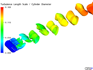
scales. This scenario is depicted in Figure 12.1, which shows that URANS models (in this case SST)
produce a single mode vortex shedding even at a relatively high
 number of
  . The vortex stream extends
far into the cylinder wake, maintaining a single frequency. This result is in
contradiction to experimental observations of a broadband turbulence
spectrum.
. The vortex stream extends
far into the cylinder wake, maintaining a single frequency. This result is in
contradiction to experimental observations of a broadband turbulence
spectrum.
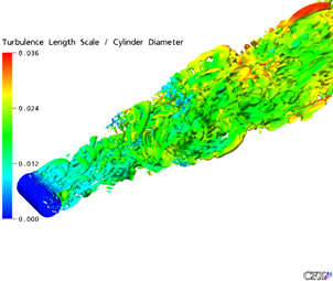
As shown in a series of publications (for example, Menter and Egorov, 2010 18, Egorov et al., 2010 6), a class of RANS models can be derived based on a theoretical concept dating back to Rotta (see Rotta, 1972 24). These models perform like standard RANS models in steady flows, but enable the formation of a broadband turbulence spectrum for certain types of unstable flows (for the types of flows, see Section 12.1.2). Such models are termed Scale-Adaptive Simulation (SAS) models. This scenario is illustrated by Figure 12.2, which shows the same simulation as in Figure 12.1 but with the SAS-SST model. The behavior seen in Figure 12.1 is therefore not inherent to all RANS models, but only to those derived in a special fashion.
The SAS concept is described in much detail in the cited references and will not
be repeated here. However, the basic model formulation must be provided for a
discussion of the model’s characteristics. The difference between standard
RANS and SAS models lies in the treatment of the scale-defining equation (typically
 -,
-,  -, or
-, or
 -equation). In classic RANS models, the scale equation
is modeled based on an analogy with the
-equation). In classic RANS models, the scale equation
is modeled based on an analogy with the  -equation using simple dimensional
arguments. The scale equation of SAS models is based on an exact transport equation
for the turbulence length scale as proposed by Rotta. This method was re-visited by
Menter and Egorov, 2010 18 and avoids some limitations
of the original Rotta model. As a result of this re-formulation, it was shown that
the second derivative of the velocity field must be included in the source terms of
the scale equation. The original SAS model (Menter and Egorov, 2010 18) was formulated as a two-equation model, with the
variable
-equation using simple dimensional
arguments. The scale equation of SAS models is based on an exact transport equation
for the turbulence length scale as proposed by Rotta. This method was re-visited by
Menter and Egorov, 2010 18 and avoids some limitations
of the original Rotta model. As a result of this re-formulation, it was shown that
the second derivative of the velocity field must be included in the source terms of
the scale equation. The original SAS model (Menter and Egorov, 2010 18) was formulated as a two-equation model, with the
variable  for the
scale equation:
for the
scale equation:
 | (12–1) |
 | (12–2) |
 | (12–3) |
The main new term is the one including the von Karman length scale
 , which does not appear in any standard RANS model. The second
velocity derivative allows the model to adjust its length scale to those structures
already resolved in the flow. This functionality is not present in standard RANS
models. This leads to the behavior shown in Figure 12.2, which agrees more closely with the experimental
observations for such flows.
, which does not appear in any standard RANS model. The second
velocity derivative allows the model to adjust its length scale to those structures
already resolved in the flow. This functionality is not present in standard RANS
models. This leads to the behavior shown in Figure 12.2, which agrees more closely with the experimental
observations for such flows.
The  term can be transformed and implemented into any other
scale-defining equation resulting in SAS capabilities as in the case of the SAS-SST
model. For the SAS-SST model, the additional term in the
term can be transformed and implemented into any other
scale-defining equation resulting in SAS capabilities as in the case of the SAS-SST
model. For the SAS-SST model, the additional term in the  -equation resulting from the transformation has been
designed to have no (or at least minimal) effect on the SST model’s RANS
performance for wall boundary layers. It can have a moderate effect on free shear
flows (Davidson, 2006 4).
-equation resulting from the transformation has been
designed to have no (or at least minimal) effect on the SST model’s RANS
performance for wall boundary layers. It can have a moderate effect on free shear
flows (Davidson, 2006 4).
The SAS model will remain in steady RANS mode for wall bounded flows, and can switch to SRS mode in flows with large and unstable separation zones (see Section 12.1.2).
Detached Eddy Simulation (DES) was introduced by Spalart and co-workers (Spalart et al., 1997 30, 2000 31, Travin et al., 2000 34, Strelets, 2001 33), to eliminate the main limitation of LES models by proposing a hybrid formulation that switches between RANS and LES based on the grid resolution provided. By this formulation, the wall boundary layers are entirely covered by the RANS model and the free shear flows away from walls are typically computed in LES mode. The formulation is mathematically relatively simple and can be built on top of any RANS turbulence model. DES has attained significant attention in the turbulence community as it was the first SRS model that allowed the inclusion of SRS capabilities into common engineering flow simulations.
Within DES models, the switch between RANS and LES is based on a criterion like the following:
 | (12–4) |
where  is the maximum edge length of
the local computational cell. The actual formulation for a two-equation model (for
example, the
is the maximum edge length of
the local computational cell. The actual formulation for a two-equation model (for
example, the  -equation of the
  model)
is:
model)
is:
 | (12–5) |
 | (12–6) |
As the grid is refined below the limit  the DES-limiter is activated and switches the model from RANS to
LES mode. For wall boundary layers, this translates into the requirement that the
RANS formulation is preserved as long as the following condition holds:
the DES-limiter is activated and switches the model from RANS to
LES mode. For wall boundary layers, this translates into the requirement that the
RANS formulation is preserved as long as the following condition holds:
 , where
  is the boundary layer
thickness. The intention of the model is to run in RANS mode for attached flow
regions, and to switch to LES mode in detached regions away from walls. This switch
suggests that the original DES formulation, as well as its later versions, require a
grid and time step resolution to be of LES quality once they switch to the grid
spacing as the defining length scale. Once the limiter is activated, the models lose
their RANS calibration and all relevant turbulence information must be resolved. For
this reason, for example in free shear flows, the DES approach offers no
computational savings over a standard LES model. However, it allows you to avoid the
high computing costs of covering the wall boundary layers in LES mode.
is the boundary layer
thickness. The intention of the model is to run in RANS mode for attached flow
regions, and to switch to LES mode in detached regions away from walls. This switch
suggests that the original DES formulation, as well as its later versions, require a
grid and time step resolution to be of LES quality once they switch to the grid
spacing as the defining length scale. Once the limiter is activated, the models lose
their RANS calibration and all relevant turbulence information must be resolved. For
this reason, for example in free shear flows, the DES approach offers no
computational savings over a standard LES model. However, it allows you to avoid the
high computing costs of covering the wall boundary layers in LES mode.
It is also important to note that the DES limiter can already be activated by grid refinement inside attached boundary layers. This is undesirable as it affects the RANS model by reducing the eddy viscosity; this can lead to Grid-Induced Separation (GIS), as discussed by Menter and Kuntz, 2002 19, where the boundary layers can separate at arbitrary locations depending on the grid spacing. In order to avoid this limitation, the DES concept has been extended to Delayed-DES (DDES) by Spalart et al., 2006 32, following the proposal of Menter and Kuntz, 2002 19 of "shielding" the boundary layer from the DES limiter. The DDES extension was also applied to the DES-SA formulation resulting in the DDES-SA model, as well as to the SST model giving the DDES-SST model.
For two-equation models, the dissipation term in the  -equation is thereby re-formulated
as follows:
-equation is thereby re-formulated
as follows:
 | (12–7) |
 | (12–8) |
The function  is designed in such a way as to give
  inside the wall boundary layer and
  away from the wall. The definition of this function is intricate
as it involves a balance between proper shielding and not suppressing the formation
of resolved turbulence as the flow separates from the wall. As the function
away from the wall. The definition of this function is intricate
as it involves a balance between proper shielding and not suppressing the formation
of resolved turbulence as the flow separates from the wall. As the function
 blends over to the LES formulation near the boundary layer edge,
no perfect shielding can be achieved. The limit for DDES is typically in the range
of
blends over to the LES formulation near the boundary layer edge,
no perfect shielding can be achieved. The limit for DDES is typically in the range
of  and therefore allows for meshes where
  is a factor of five smaller
than for DES, without negative effects on the RANS-covered boundary layer. However,
even this limit is frequently reached and GIS can appear even with DDES.
is a factor of five smaller
than for DES, without negative effects on the RANS-covered boundary layer. However,
even this limit is frequently reached and GIS can appear even with DDES.
There are a number of DDES models available in Ansys CFD. They follow the same principal idea with respect to switching between RANS and LES mode. The models differ therefore mostly by their RANS capabilities and should be selected accordingly.
The SDES formulation is a member of the DDES model family, but offers alternatives for the shielding function and the definition of the grid scale. The impact on the turbulence model is, as usual, formulated as an additional sink term in the k-equation:
 | (12–9) |
The shielding function  provides much stronger shielding than the corresponding
  function above. For this reason, the natural
shielding of the model based on the mesh length definition,
function above. For this reason, the natural
shielding of the model based on the mesh length definition,  , can be reduced. The mesh
length scale used in the SDES model is defined as follows:
, can be reduced. The mesh
length scale used in the SDES model is defined as follows:
 | (12–10) |
The first part represents the conventional LES grid length scale definition, and the second part is again based on the maximum edge length as in the DES formulation. However, the factor 0.2 ensures that for highly stretched meshes, the grid length scale is a factor of 5 smaller than for DES/DDES. Since the grid length scale enters quadratically into the definition of the eddy viscosity in LES mode, this means a reduction by a factor of 25 in such cases. It will be shown that this drastically reduces the frequently observed problem of slow ‘transition’ of DES/DDES models from RANS to LES. Note that the combination of this more ‘aggressive’ length scale with the conventional DDES shielding function would severely reduce the shielding properties of DDES and is therefore not recommended.
The SDES constant  is also
different from in the DES/DDES formulation, where it is calibrated based on decaying
isotropic turbulence (DIT) with the goal of matching the turbulence spectrum
relative to data after certain running times. However, in engineering flows, one
typically has to deal with shear flows, for which a reduced Smagorinsky constant
should be used. This is achieved by setting
is also
different from in the DES/DDES formulation, where it is calibrated based on decaying
isotropic turbulence (DIT) with the goal of matching the turbulence spectrum
relative to data after certain running times. However, in engineering flows, one
typically has to deal with shear flows, for which a reduced Smagorinsky constant
should be used. This is achieved by setting  =0.4. The
combination of the re-definition of the grid length scale and the modified constant
leads to a reduction in the eddy viscosity by a factor of around 60 in separating
shear flows on stretched grids. It will be shown later that this results in a much
more rapid transition from RANS to LES.
=0.4. The
combination of the re-definition of the grid length scale and the modified constant
leads to a reduction in the eddy viscosity by a factor of around 60 in separating
shear flows on stretched grids. It will be shown later that this results in a much
more rapid transition from RANS to LES.
The shielding function  is formulated such that it provides essentially asymptotic shielding on any grid. In
flat plate tests, the limit was pushed below
is formulated such that it provides essentially asymptotic shielding on any grid. In
flat plate tests, the limit was pushed below  .
.
The following test case shows the improved shielding properties of SDES/SBES
models relative to DDES. The flow is a diffuser flow in an axisymmetric geometry
featuring a small separation bubble. Due to the adverse pressure gradient, the
boundary layer grows strongly and shielding is difficult to achieve due to the
strong increase in  .
.
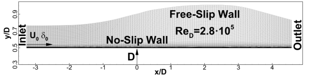
The computational domain is shown in Figure 12.3: The domain and grid for the separated flow in CS0 diffuser. The
length of the domain in the streamwise direction is about
7.8· [m] (
[m] ( is the diameter of the cylinder and
  corresponds to the separation point in the experiment). For this flow, a standard
RANS grid is used with steps in the streamwise and circumferential directions of
corresponds to the separation point in the experiment). For this flow, a standard
RANS grid is used with steps in the streamwise and circumferential directions of  and
and  respectively (the grid step in the
circumferential direction is changing in the radial direction due to the
axisymmetric geometry). Here
respectively (the grid step in the
circumferential direction is changing in the radial direction due to the
axisymmetric geometry). Here  is the boundary layer thickness at the
inlet section. The height of the wall cell is chosen to satisfy the condition
is the boundary layer thickness at the
inlet section. The height of the wall cell is chosen to satisfy the condition
 in the entire domain and around 30 cells cover the
boundary layer.
in the entire domain and around 30 cells cover the
boundary layer.
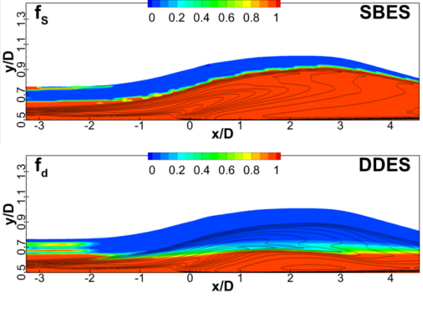
As seen from the contours of the SBES and DDES blending functions shown in Figure 12.4: Contours of blending functions overset by vorticity iso-lines for CS=0 diffuser for SBES and DDES models, SBES covers the entire boundary layer including the rapid growth area of the boundary layer due to the separation bubble, while DDES preserves only the portion of the domain at the inlet. This means that under adverse pressure gradient conditions, the shielding properties of DDES are substantially impaired.
Figure 12.4: Contours of blending functions overset by vorticity iso-lines for CS=0 diffuser for SBES and DDES models
Similar observations can be made for the eddy viscosity fields shown in Figure 12.5: Contours of eddy viscosity ratio for CS0 diffuser for SBES and DDES models. The eddy viscosity levels of SBES correspond to those of the SST model (not shown), while the DDES model produces much reduced levels in the adverse pressure gradient region.
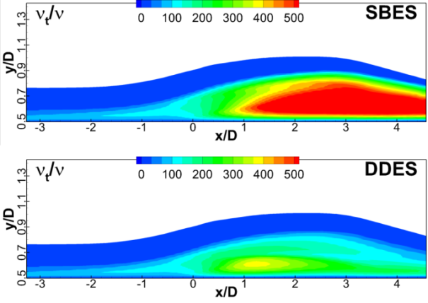
As stated in the introduction, the SBES model concept is built on the SDES
formulation. In addition to SDES, SBES is using the shielding function
 to explicitly switch between different turbulence model formulations in RANS and LES
modes. In general terms, that means for the turbulence stress tensor:
to explicitly switch between different turbulence model formulations in RANS and LES
modes. In general terms, that means for the turbulence stress tensor:
 | (12–11) |
where  is the RANS part and
  is the LES
part of the modeled stress tensor. In case both model portions are based on
eddy-viscosity concepts, the formulation simplifies to:
is the LES
part of the modeled stress tensor. In case both model portions are based on
eddy-viscosity concepts, the formulation simplifies to:
 | (12–12) |
Such a formulation would not be feasible without strong shielding. When using the conventional shielding functions from the DDES model, the corresponding model would not be able to maintain a zero pressure gradient RANS boundary layer on any grid.
The SBES model formulation is currently recommended relative to other global hybrid RANS-LES methods. It offers the following advantages:
Asymptotic shielding of the RANS boundary layers
Explicit switch to user-specified LES model in LES region
Rapid ‘transition’ from RANS to LES region
Clear visualization of RANS and LES regions based on shielding function
Wall-modeled LES capability once in LES/WMLES mode
The details of different LES models can be found in the User and Theory documentation of the corresponding solvers. As described in Section 12.1.1.5.1, the main purpose of LES models is to provide sufficient damping for the smallest (unresolved) scales. For this reason, it is not advisable to use complex formulations, but to stay with simple algebraic models. The most widely used LES model is the Smagorinsky, 1963 29 model:
 | (12–13) |
The main deficiency of the Smagorinsky model is that its eddy-viscosity does not
go to zero for laminar shear flows (only  ). For this reason, this model also requires a near-wall damping
function in the viscous sublayer. It is desirable to have a LES formulation that
automatically provides zero eddy-viscosity for simple laminar shear flows. This is
especially important when computing flows with laminar turbulent transition, where
the Smagorinsky model would negatively affect the laminar flow. The simplest model
to provide this functionality is the WALE (Wall-Adapting Local Eddy-viscosity) model
of Nicoud and Ducros, 1999 22. The same effect is also
achieved by dynamic LES models, but at the cost of a somewhat higher complexity.
None of the classical LES models addresses the main industrial problem of excessive
computing costs for wall-bounded flows at moderate to high Reynolds numbers.
). For this reason, this model also requires a near-wall damping
function in the viscous sublayer. It is desirable to have a LES formulation that
automatically provides zero eddy-viscosity for simple laminar shear flows. This is
especially important when computing flows with laminar turbulent transition, where
the Smagorinsky model would negatively affect the laminar flow. The simplest model
to provide this functionality is the WALE (Wall-Adapting Local Eddy-viscosity) model
of Nicoud and Ducros, 1999 22. The same effect is also
achieved by dynamic LES models, but at the cost of a somewhat higher complexity.
None of the classical LES models addresses the main industrial problem of excessive
computing costs for wall-bounded flows at moderate to high Reynolds numbers.
There are numerous cases at very low Reynolds numbers where LES can be an
industrial option. Under such conditions, the wall boundary layers are likely
laminar and turbulence forms only in separated shear layers and detached flow
regions. Such situations can be identified by analyzing RANS eddy viscosity
solutions for a given flow. In the case where the ratio of turbulence to molecular
viscosity  is smaller than
  inside the boundary layer, it can be assumed that the boundary layers are laminar
and no resolution of near-wall turbulence is required. Such conditions are observed
for flows around valves or other small-scale devices at low Reynolds numbers.
inside the boundary layer, it can be assumed that the boundary layers are laminar
and no resolution of near-wall turbulence is required. Such conditions are observed
for flows around valves or other small-scale devices at low Reynolds numbers.
LES can also be applied to free shear flows, where resolution requirements are much reduced relative to wall-bounded flows.
In order to understand the motivation for hybrid models, one has to discuss the limitations of Large Eddy Simulation (LES). LES has been the most widely used SRS model over the last decades. It is based on the concept of resolving only the large scales of turbulence and to model the small scales. The classical motivation for LES is that the large scales are problem-dependent and difficult to model, whereas the smaller scales become more and more universal and isotropic and can be modeled more easily.
LES is based on filtering the Navier-Stokes equations over a finite spatial region (typically the grid volume) and aimed at only resolving the portions of turbulence larger than the filter width. Turbulence structures smaller than the filter are then modeled, typically by a simple Eddy Viscosity model.
The filtering operation is defined as:
 | (12–14) |
where  is the spatial filter. Filtering the Navier-Stokes equations
results in the following form (density fluctuations neglected):
is the spatial filter. Filtering the Navier-Stokes equations
results in the following form (density fluctuations neglected):
 | (12–15) |
The equations feature an additional stress term due to the filtering operation:
 | (12–16) |
Despite the difference in derivation, the additional sub-grid stress tensor is typically modeled as in RANS using an eddy viscosity model:
 | (12–17) |
The important practical implication from this modeling approach is that the modeled momentum equations for RANS and LES are identical if an eddy-viscosity model is used in both cases. The modeled Navier-Stokes equations have no knowledge of their derivation. The only information they obtain from the turbulence model is the level of the eddy viscosity. Depending on that, the equations will operate in RANS or LES mode (or in some intermediate mode). The formal identity of the filtered Navier-Stokes and the RANS equations is the basis of hybrid RANS-LES turbulence models, which can obviously be introduced into the same set of momentum equations. Only the model (and the numerics) have to be switched.
Classical LES models are of the form of the Smagorinsky, 1963 29 model:
 | (12–18) |
where  is a measure of the grid spacing of the numerical
mesh,
is a measure of the grid spacing of the numerical
mesh,  is the strain rate scalar and
  is a constant. This is obviously a rather simple
formulation, indicating that LES models will not provide a highly accurate
representation of the smallest scales. From a practical standpoint, a very
detailed modeling might not be required. A more appropriate goal for LES is not
to model the impact of the unresolved scales onto the resolved ones, but to
model the dissipation of the smallest resolved scales. This can be seen from
Figure 12.6 showing the
turbulence energy spectrum of a Decaying Isotropic Turbulence (DIT) test case;
that is, initially stirred turbulence in a box, decaying over time (Comte-Bellot
and Corrsin, 1971 3).
is a constant. This is obviously a rather simple
formulation, indicating that LES models will not provide a highly accurate
representation of the smallest scales. From a practical standpoint, a very
detailed modeling might not be required. A more appropriate goal for LES is not
to model the impact of the unresolved scales onto the resolved ones, but to
model the dissipation of the smallest resolved scales. This can be seen from
Figure 12.6 showing the
turbulence energy spectrum of a Decaying Isotropic Turbulence (DIT) test case;
that is, initially stirred turbulence in a box, decaying over time (Comte-Bellot
and Corrsin, 1971 3).  is the turbulence
energy as a function of wave number
is the turbulence
energy as a function of wave number  . Small
  values represent large
eddies and large
values represent large
eddies and large  values represent small eddies. Turbulence moves
down the turbulence spectrum from the small wave number to the high wave
numbers. In a fully resolved simulation (Direct Numerical Simulation, or DNS),
the turbulence is dissipated into heat at the smallest scales
(
values represent small eddies. Turbulence moves
down the turbulence spectrum from the small wave number to the high wave
numbers. In a fully resolved simulation (Direct Numerical Simulation, or DNS),
the turbulence is dissipated into heat at the smallest scales
( in Figure 12.6), by viscosity.
The dissipation is achieved by:
in Figure 12.6), by viscosity.
The dissipation is achieved by:
 | (12–19) |
where  is typically a very small
kinematic molecular viscosity. The dissipation
is typically a very small
kinematic molecular viscosity. The dissipation  is
still of finite value as the velocity gradients of the smallest scales are very
large.
is
still of finite value as the velocity gradients of the smallest scales are very
large.
LES computations are usually performed on numerical grids that are too coarse
to resolve the smallest scales. In the current example, the cut-off limit of LES
(resolution limit) is at around  . The
velocity gradients of the smallest resolved scales in LES are therefore much
smaller than those at the DNS limit. The molecular viscosity is then not
sufficient to provide the correct level of dissipation. In this case, the proper
amount of dissipation can be achieved by increasing the viscosity, using an
eddy-viscosity:
. The
velocity gradients of the smallest resolved scales in LES are therefore much
smaller than those at the DNS limit. The molecular viscosity is then not
sufficient to provide the correct level of dissipation. In this case, the proper
amount of dissipation can be achieved by increasing the viscosity, using an
eddy-viscosity:
 | (12–20) |
The eddy viscosity is calibrated to provide the correct amount of dissipation at the LES grid limit. The effect can be seen in Figure 12.6, where a LES of the DIT case is performed without a LES model and with different LES models. When the LES models are activated, the energy is dissipated and the models provide a sensible spectrum for all resolved scales. LES is not modeling the influence of unresolved small scale turbulence onto the larger, resolved scales, but the dissipation of turbulence into heat (the dissipated energy is typically very small relative to the thermal energy of the fluid and does not have to be accounted for, except for high Mach number flows).
Figure 12.6: Turbulence spectrum for DIT test case after t=2. Comparison of results without Sub-Grid Scale model (no LES) with WALE and Smagorinsky LES model simulations
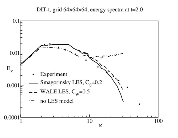
This discussion shows that LES is a fairly simple technology, which does not provide a reliable backbone for modeling. This is also true for more complex LES models like dynamic models. Dynamic eddy viscosity LES models (see Geurts, 2004 12) are designed to estimate the required level of dissipation at the grid limit from flow conditions at larger scales (typically twice the filter width), thereby reducing the need for model calibration. Such models, however, also only provide a suitable eddy viscosity level for energy dissipation. As a result, within the LES framework, all features and effects of the flow that are of interest and relevance to engineers have to be resolved in space and time. This requirement makes LES a very CPU-expensive technology.
Even more demanding is the application of LES to wall-bounded flows, which is
the typical situation in engineering flows. The turbulent length scale,
 , of the large eddies can be expressed as:
 | (12–21) |
where  is the wall distance and
  a constant. Even the
(locally) largest scales become very small near the wall and require a high
resolution in all three space dimensions and in time.
a constant. Even the
(locally) largest scales become very small near the wall and require a high
resolution in all three space dimensions and in time.
The linear dependence of  on
on  indicates that the turbulence
length scales approach zero near the wall, which would require an infinitely
fine grid to resolve them. This is not the case in reality, as the molecular
viscosity prevents scales smaller than the Kolmogorov limit. This is manifested
by the viscous or laminar sublayer, a region very close to the wall, where
turbulence is damped and does not need to be resolved. However, the viscous
sublayer thickness is a function of the Reynolds number, Re, of the flow. At
higher Re numbers, the viscous sublayer becomes decreasingly thinner and thereby
allows the survival of smaller and smaller eddies, which need to be resolved.
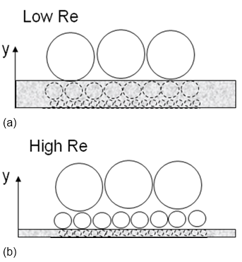
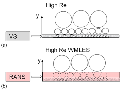
This is depicted in Figure 12.7 showing a sketch of turbulence structures in the vicinity of the wall (for
example, channel flow with flow direction normal to observer). The upper part of
the picture represents a low Re number and the lower part a higher Re number
situation. The gray box indicates the viscous sublayer for the two Re numbers.
The structures inside the viscous sublayer (circles inside the gray box) are
depicted but not present in reality due to viscous damping. Only the structures
outside of the viscous sublayer (that is, above the gray box) exist and need to
be resolved. Due to the reduced thickness of the viscous sublayer in the high Re
case, substantially more resolution is required to resolve all active scales.
Wall-resolved LES is therefore prohibitively expensive for moderate to high
Reynolds numbers. This is the main reason why LES is not suitable for most
engineering flows.
indicates that the turbulence
length scales approach zero near the wall, which would require an infinitely
fine grid to resolve them. This is not the case in reality, as the molecular
viscosity prevents scales smaller than the Kolmogorov limit. This is manifested
by the viscous or laminar sublayer, a region very close to the wall, where
turbulence is damped and does not need to be resolved. However, the viscous
sublayer thickness is a function of the Reynolds number, Re, of the flow. At
higher Re numbers, the viscous sublayer becomes decreasingly thinner and thereby
allows the survival of smaller and smaller eddies, which need to be resolved.
This is depicted in Figure 12.7 showing a sketch of turbulence structures in the vicinity of the wall (for
example, channel flow with flow direction normal to observer). The upper part of
the picture represents a low Re number and the lower part a higher Re number
situation. The gray box indicates the viscous sublayer for the two Re numbers.
The structures inside the viscous sublayer (circles inside the gray box) are
depicted but not present in reality due to viscous damping. Only the structures
outside of the viscous sublayer (that is, above the gray box) exist and need to
be resolved. Due to the reduced thickness of the viscous sublayer in the high Re
case, substantially more resolution is required to resolve all active scales.
Wall-resolved LES is therefore prohibitively expensive for moderate to high
Reynolds numbers. This is the main reason why LES is not suitable for most
engineering flows.
Figure 12.7: Sketch of turbulence structures for wall-bounded channel flow with viscous sublayer (a) Low Re number (b) High Re number (Grey area: viscous sublayer)
The Reynolds number dependence of wall-resolved LES can be estimated for a
simple periodic channel flow as shown in Figure 12.8 ( -streamwise,
  -wall-normal,
  -spanwise,
  is the channel height).
 | (12–22) |
The typical resolution requirements for LES are:
 | (12–23) |
where  is
the non-dimensional grid spacing in the streamwise direction,
is
the non-dimensional grid spacing in the streamwise direction,  in the spanwise and
  the number of cells across half of the channel
height. With the definitions:
the number of cells across half of the channel
height. With the definitions:
 | (12–24) |
one can find the number,  of cells required as a function of
  ,
for resolving this limited domain of simple flow (see Table 12.1).
,
for resolving this limited domain of simple flow (see Table 12.1).
 | (12–25) |


(For the practitioner: the Reynolds,  , number based on
the bulk velocity is around a factor of ten larger than the Reynolds number,
, number based on
the bulk velocity is around a factor of ten larger than the Reynolds number,
 , based on friction
velocity. Note that
, based on friction
velocity. Note that  is based on
  ). The number of cells increases strongly with
 number, demanding high computing
resources even for very simple flows. The CPU power scales even less favorably,
as the time step must also be reduced to maintain a constant CFL number
(
number, demanding high computing
resources even for very simple flows. The CPU power scales even less favorably,
as the time step must also be reduced to maintain a constant CFL number
( ).
).
The Re number scaling for channel flows could be reduced by the application of
wall functions with increasing  values for higher
  numbers. However,
wall functions are a strong source of modeling uncertainty and can undermine the
overall accuracy of simulations. Furthermore, the experience with RANS models
shows that the generation of high quality wall-function grids for complex
geometries is a very challenging task. This task is even more challenging for
LES applications, where you would have to control the resolution in all three
space dimensions to conform to the LES requirements (for example,
numbers. However,
wall functions are a strong source of modeling uncertainty and can undermine the
overall accuracy of simulations. Furthermore, the experience with RANS models
shows that the generation of high quality wall-function grids for complex
geometries is a very challenging task. This task is even more challenging for
LES applications, where you would have to control the resolution in all three
space dimensions to conform to the LES requirements (for example,
 and
and  then depend on
  ).
).
For external flows, there is an additional Re number effect resulting from the relative thickness of the boundary layer (for example, boundary layer thickness relative to chord length of an airfoil). At high Re numbers, the boundary layer becomes very thin relative to the body’s dimensions. Assuming a constant resolution per boundary layer volume, Spalart et al., 1997 30, 2000 31 provided estimates of computing power requirements for high Reynolds number aerodynamic flows under the most favorable assumptions. Even then, the computing resources are excessive and will not be met even by optimistic estimates of computing power increases for several decades, except for simple flows.
While the computing requirements for high Re number flows are dominated by the relatively thin boundary layers, the situation for low Re number technical flows is often equally unfavorable, as effects such as laminar-turbulent transition dominate and need to be resolved. Based on reduced geometry simulations of turbomachinery blades (see Michelassi, 2003 20), an estimate for a single turbine blade with end-walls is given in Table 12.2.
Table 12.2: Computing power estimate for a single turbomachinery blade with end-walls
|
Method |
Cells |
Time steps |
Inner loops per time step |
Ratio to RANS |
|---|---|---|---|---|
|
RANS |
~106 |
~102 |
1 |
1 |
|
LES |
~108–109 |
~104–105 |
10 |
105–107 |
Considering that the goal of turbomachinery companies is the simulation of
entire machines (or at least significant parts of them), it is unrealistic to
assume that LES will become a major element of industrial CFD simulations even
for such low Re number ( )
applications. However, LES can play a role in the detailed analysis of elements
of such flows like cooling holes or active flow control.
)
applications. However, LES can play a role in the detailed analysis of elements
of such flows like cooling holes or active flow control.
All the above does not mean that LES of wall-bounded flows is not feasible at
all, but just that the costs of such simulations are high. Figure 12.9 shows the grid used
for a LES around a NACA 0012 airfoil using the WALE model. The computational
domain is limited in the spanwise direction to 5% of the airfoil chord length
using periodic boundary conditions in that direction. At a Reynolds number of  a spanwise extent of 5% has been estimated as the minimum
domain size that allows turbulence structures to develop without being
synchronized across the span by the periodic boundary conditions. The estimate
was based on the boundary layer thickness at the trailing edge as obtained from
a precursor RANS computation. This boundary layer thickness is about 2% chord
length. The grid had 80 cells in the spanwise direction and overall
a spanwise extent of 5% has been estimated as the minimum
domain size that allows turbulence structures to develop without being
synchronized across the span by the periodic boundary conditions. The estimate
was based on the boundary layer thickness at the trailing edge as obtained from
a precursor RANS computation. This boundary layer thickness is about 2% chord
length. The grid had 80 cells in the spanwise direction and overall
 cells. The simulation was carried out at an angle of attack of
 ,
using Ansys Fluent in incompressible mode. The chord length was set to
,
using Ansys Fluent in incompressible mode. The chord length was set to
 , the freestream velocity,
  and
the fluid is air at standard conditions. The time step was set to
and
the fluid is air at standard conditions. The time step was set to  giving a Courant number of
  inside the boundary layer. Figure 12.10 shows turbulence
structures near the leading edge (a) and the trailing edge (b). Near the leading
edge, the laminar-turbulent transition can clearly be seen. The transition is
triggered by a laminar separation bubble. Near the trailing edge, the turbulence
structures are already relatively large, but still appear unsynchronized in the
spanwise direction (no large scale 2D structures with axis orientation in the
spanwise direction). The simulation was run for ~104
time steps before the averaging procedure was started. The time averaging was
conducted for
inside the boundary layer. Figure 12.10 shows turbulence
structures near the leading edge (a) and the trailing edge (b). Near the leading
edge, the laminar-turbulent transition can clearly be seen. The transition is
triggered by a laminar separation bubble. Near the trailing edge, the turbulence
structures are already relatively large, but still appear unsynchronized in the
spanwise direction (no large scale 2D structures with axis orientation in the
spanwise direction). The simulation was run for ~104
time steps before the averaging procedure was started. The time averaging was
conducted for  time steps. Figure 12.11 shows
a comparison of the wall pressure coefficient
time steps. Figure 12.11 shows
a comparison of the wall pressure coefficient  and Figure 12.12 of the wall
shear stress coefficient
and Figure 12.12 of the wall
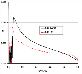
shear stress coefficient  on the suction side of the airfoil in comparison to a RANS
computation using the SST model (Menter, 1994 16).
No detailed discussion of the simulation is intended here, but the comparison of
the wall shear stress with the well-calibrated RANS model indicates that the
resolution of the grid is still insufficient for capturing the near-wall
details. For this reason, the wall shear stress is significantly underestimated
by about 30% compared to the SST model in the leading edge area. As the trailing
edge is approached, the comparison improves, mainly because the boundary layer
thickness is increased whereas the wall shear stress is decreased, which
produces a higher relative resolution in the LES. Based on this simulation, it
is estimated that a refinement by a factor of 2, in both streamwise and spanwise
directions, would be required in order to reproduce the correct wall shear
stress. While such a resolution is not outside the realm of available computers,
it is still far too high for day-to-day simulations of more complex configurations.
on the suction side of the airfoil in comparison to a RANS
computation using the SST model (Menter, 1994 16).
No detailed discussion of the simulation is intended here, but the comparison of
the wall shear stress with the well-calibrated RANS model indicates that the
resolution of the grid is still insufficient for capturing the near-wall
details. For this reason, the wall shear stress is significantly underestimated
by about 30% compared to the SST model in the leading edge area. As the trailing
edge is approached, the comparison improves, mainly because the boundary layer
thickness is increased whereas the wall shear stress is decreased, which
produces a higher relative resolution in the LES. Based on this simulation, it
is estimated that a refinement by a factor of 2, in both streamwise and spanwise
directions, would be required in order to reproduce the correct wall shear
stress. While such a resolution is not outside the realm of available computers,
it is still far too high for day-to-day simulations of more complex configurations.
Figure 12.9: Details of grid around a NACA 0012 airfoil (a) Grid topology (b) Leading edge area (c) Trailing edge area
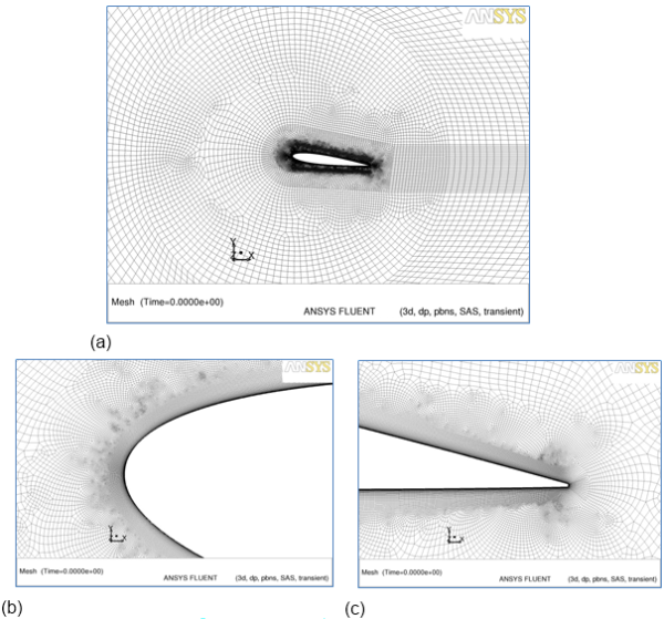
Figure 12.10: Turbulence structures of WALE LES computation around a NACA 0012 airfoil (a) Leading edge (b) Trailing edge (Q-criterion, color- spanwise velocity component)
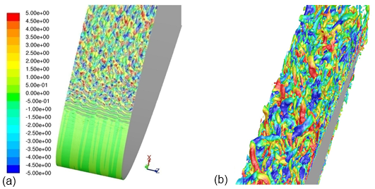
Figure 12.11: Wall pressure coefficient Cp on the suction side of a NACA 0012 airfoil: comparison of RANS-SST and LES-WALE results

Figure 12.12: Wall shear stress coefficient Cf on the suction side of a NACA 0012 airfoil: comparison of RANS-SST and LES-WALE results
Overall, LES for industrial flows will be restricted in the foreseeable future to flows not involving wall boundary layers, or wall-bounded flows in strongly reduced geometries, preferentially at low Re numbers.
The limitations of the conventional LES approach are the driving force behind the development of hybrid RANS-LES models that are described in the later parts of this document.
Wall Modeled LES (WMLES) is an alternative to classical LES and reduces the
stringent and  number-dependent grid resolution
requirements of classical wall-resolved LES (Section 12.1.1.5.1) The principle idea is depicted in Figure 12.13. As described in Section 12.1.1.5.1, the near-wall turbulence
length scales increase linearly with the wall distance, resulting in smaller and
smaller eddies as the wall is approached. This effect is limited by molecular
viscosity, which damps out eddies inside the viscous sublayer (VS). As the
number-dependent grid resolution
requirements of classical wall-resolved LES (Section 12.1.1.5.1) The principle idea is depicted in Figure 12.13. As described in Section 12.1.1.5.1, the near-wall turbulence
length scales increase linearly with the wall distance, resulting in smaller and
smaller eddies as the wall is approached. This effect is limited by molecular
viscosity, which damps out eddies inside the viscous sublayer (VS). As the
 number increases,
smaller and smaller eddies appear, since the viscous sublayer becomes thinner. In
order to avoid the resolution of these small near-wall scales, RANS and LES models
are combined such that the RANS model covers the very near-wall layer, and then
switches over to the LES formulation once the grid spacing becomes sufficient to
resolve the local scales. This is seen in Figure 12.13 (b), where the RANS layer extends outside of
the VS, thus avoiding the need to resolve the inner second row of eddies depicted in
the sketch.
number increases,
smaller and smaller eddies appear, since the viscous sublayer becomes thinner. In
order to avoid the resolution of these small near-wall scales, RANS and LES models
are combined such that the RANS model covers the very near-wall layer, and then
switches over to the LES formulation once the grid spacing becomes sufficient to
resolve the local scales. This is seen in Figure 12.13 (b), where the RANS layer extends outside of
the VS, thus avoiding the need to resolve the inner second row of eddies depicted in
the sketch.
The WMLES formulation in Ansys CFD is based on the formulation of Shur et al., 2008 26:
 | (12–26) |
where  is the wall distance,
  is the von Karman constant,
  is the strain rate and
  is a near-wall damping function. This formulation was adapted to suit the needs of
the Ansys general purpose CFD codes. Near the wall, the min-function selects the
Prandtl mixing length model whereas away from the wall it switches over to the
Smagorinsky model. Meshing requirements for the WMLES approach are given in Section 12.1.2.3.3.
is a near-wall damping function. This formulation was adapted to suit the needs of
the Ansys general purpose CFD codes. Near the wall, the min-function selects the
Prandtl mixing length model whereas away from the wall it switches over to the
Smagorinsky model. Meshing requirements for the WMLES approach are given in Section 12.1.2.3.3.
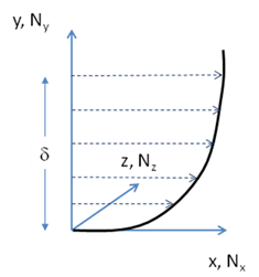
For wall boundary layer flows, the resolution requirements of WMLES depend on the
details of the model formulation. In Ansys Fluent and Ansys CFX they are (assuming for
this estimate that  is the streamwise,
  the wall normal and
  the spanwise direction as shown in
Figure 12.14):
the spanwise direction as shown in
Figure 12.14):
 | (12–27) |
where  ,
,  , and
, and  are the numbers of cells per boundary layer thickness,
  , in the streamwise, wall
normal, and spanwise directions respectively, (see Figure 12.14). About 6000-8000 cells
are needed to cover one boundary layer volume
, in the streamwise, wall
normal, and spanwise directions respectively, (see Figure 12.14). About 6000-8000 cells
are needed to cover one boundary layer volume  . This is also the minimal resolution for classical LES models at
low Reynolds numbers. Actually, for low Reynolds numbers, WMLES turns essentially
into classical LES. The advantage of WMLES is that the resolution requirements
relative to the boundary layer thickness remain independent of the Reynolds
number.
. This is also the minimal resolution for classical LES models at
low Reynolds numbers. Actually, for low Reynolds numbers, WMLES turns essentially
into classical LES. The advantage of WMLES is that the resolution requirements
relative to the boundary layer thickness remain independent of the Reynolds
number.
While WMLES is largely Reynolds number-independent for channel and pipe flows
(where the boundary layer thickness must be replaced by half of the channel height)
there remains a Reynolds number sensitivity for aerodynamic boundary layer flows,
where, the ratio of the boundary layer thickness,  , to a characteristic body dimension,
  , is decreasing with increasing
Reynolds number. In aerodynamic boundary layer flows, there are more boundary layer
volumes to consider at increased Reynolds numbers. It should also be noted that
despite the large cost savings of WMLES compared to wall-resolved LES, the cost
increase relative to RANS models is still substantial. Typical RANS computations
feature only one cell per boundary layer thickness in streamwise and spanwise
directions (
, is decreasing with increasing
Reynolds number. In aerodynamic boundary layer flows, there are more boundary layer
volumes to consider at increased Reynolds numbers. It should also be noted that
despite the large cost savings of WMLES compared to wall-resolved LES, the cost
increase relative to RANS models is still substantial. Typical RANS computations
feature only one cell per boundary layer thickness in streamwise and spanwise
directions ( ). In addition, RANS
steady-state simulations can be converged in the order of
~102–103
iterations, whereas unsteady simulations typically require
~104–105.
). In addition, RANS
steady-state simulations can be converged in the order of
~102–103
iterations, whereas unsteady simulations typically require
~104–105.
For wall-normal resolution in WMLES, it is recommended that you use grids with
 at the wall. If this cannot be achieved,
the WMLES model is formulated to tolerate coarser
at the wall. If this cannot be achieved,
the WMLES model is formulated to tolerate coarser  values (
 -insensitive
formulation) as well.
-insensitive
formulation) as well.
Figure 12.14: Sketch of boundary layer profile with thickness  , x-streamwise direction,
y-normal direction, and z-spanwise direction
, x-streamwise direction,
y-normal direction, and z-spanwise direction
For channel and pipe flows, the above resolution requirements for the boundary
layer should be applied, only replacing the boundary layer thickness,
 , with half the channel height, or with the pipe
radius in the grid estimation. This estimate would result in a minimum of ~120 cells
in the circumferential direction (
, with half the channel height, or with the pipe
radius in the grid estimation. This estimate would result in a minimum of ~120 cells
in the circumferential direction ( ) for a
fully developed pipe flow.
) for a
fully developed pipe flow.
It should be noted that reductions in grid resolution similar to WMLES can be
achieved with classical LES models when using LES wall functions. However, the
generation of suitable grids for LES wall functions is very challenging as the grid
spacing normal to the wall and the wall-parallel grid resolution requirements are
coupled and strongly dependent on  number (unlike RANS where only the
wall-normal resolution must be considered).
number (unlike RANS where only the
wall-normal resolution must be considered).
In Ansys Fluent, the WMLES formulation can be selected as one of the LES options; in Ansys CFX it is always activated inside the LES zone of the Zonal Forced LES (ZFLES) method.
The idea behind ELES is to predefine different zones with different treatments of turbulence in the preprocessing stage. The domain is split into a RANS and a LES portion ahead of the simulation. Between the different regions, the turbulence model is switched from RANS to LES/WMLES. In order to maintain consistency, synthetic turbulence is generally introduced at RANS-LES interfaces. ELES is actually not a new model, but an infrastructure that combines existing elements of technology in a zonal fashion. The recommendations for each zone are therefore the same as those applicable to the individual models.
In Ansys Fluent, an Embedded LES formulation is available (Cokljat et al., 2009 2). It allows the combination of most RANS models with all non-dynamic LES models in the predefined RANS and LES regions respectively. The conversion from modeled turbulence to resolved turbulence is achieved at the RANS-LES interface using the Vortex Method (Mathey et al., 2003 15).
In CFX, a similar functionality is achieved using a method called Zonal Forced LES (ZFLES) (Menter et al., 2009 17). The simulation is based on a pre-selected RANS model. In a LES zone, specified via a CEL expression, forcing terms in the momentum and turbulence equations are activated. These terms push the RANS model into a WMLES formulation. In addition, synthetic turbulence is generated at the RANS-LES interface,
There is an additional option in Ansys Fluent that involves using a global turbulence model (SAS, DDES, SDES, SBES), and activates the generation of synthetic turbulence at a pre-defined interface. The code takes care of balancing the resolved and modeled turbulence through the interface. This option can be used to force global hybrid models into unsteadiness for cases where the natural flow instability is not sufficient. Unlike ELES, the same turbulence model is used upstream and downstream of the interface. In ELES, different models are used in different zones on opposite sides of the interface.
Such forcing can also be achieved in Ansys CFX by specifying a thin LES region and using the SAS or SBES model globally. The SBES model is most suitable for this scenario.
Classical LES requires providing unsteady fluctuations at turbulent
inlets/interfaces (RANS-LES interface) to the LES domain. This makes LES
substantially more demanding than RANS, where profiles of the mean turbulence
quantities ( and
and  or
or  and
and  ) are typically specified. An example is a fully
turbulent channel (pipe) flow. The flow enters the domain in a fully turbulent state
at the inlet, so you are therefore required to provide suitable resolved turbulence
at such an inlet location through unsteady inlet velocity profiles. The inlet
profiles have to be composed in such a way that their time average corresponds to
the correct mean flow inlet profiles, as well as to all relevant turbulence
characteristics (turbulence time and length scales, turbulence stresses, and so on).
For fully turbulent channel and pipe flows, this requirement can be circumvented by
the application of periodic boundary conditions in the flow direction. The flow is
thereby driven by a source term in the momentum equation acting in the streamwise
direction. By that trick, the turbulence leaving the domain at the outlet enters the
domain again at the inlet, thereby avoiding the explicit specification of unsteady
turbulence profiles. This approach can be employed only for very simple
configurations. It requires a sufficient length of the domain (at least
~8–10h, see Figure 12.8) in
the streamwise direction to enable the formation inside the domain of turbulence
structures independent of the periodic boundaries.
) are typically specified. An example is a fully
turbulent channel (pipe) flow. The flow enters the domain in a fully turbulent state
at the inlet, so you are therefore required to provide suitable resolved turbulence
at such an inlet location through unsteady inlet velocity profiles. The inlet
profiles have to be composed in such a way that their time average corresponds to
the correct mean flow inlet profiles, as well as to all relevant turbulence
characteristics (turbulence time and length scales, turbulence stresses, and so on).
For fully turbulent channel and pipe flows, this requirement can be circumvented by
the application of periodic boundary conditions in the flow direction. The flow is
thereby driven by a source term in the momentum equation acting in the streamwise
direction. By that trick, the turbulence leaving the domain at the outlet enters the
domain again at the inlet, thereby avoiding the explicit specification of unsteady
turbulence profiles. This approach can be employed only for very simple
configurations. It requires a sufficient length of the domain (at least
~8–10h, see Figure 12.8) in
the streamwise direction to enable the formation inside the domain of turbulence
structures independent of the periodic boundaries.
In most practical cases, the geometry does not enable fully periodic simulations. It can however feature fully developed profiles at the inlet (again typically pipe/channel flows). In such cases, you can perform a periodic precursor simulation on a separate periodic domain and then insert the unsteady profiles obtained at any cross-section of that simulation to the inlet of the complex CFD domain. This approach requires either a direct coupling of two separate CFD simulations or the storage of a sufficient number of unsteady profiles from the periodic simulation to be read in by the full simulation.
In a real situation, however, the inlet profiles might not be fully developed and no simple method exists for producing consistent inlet turbulence. In such cases, synthetic turbulence can be generated, based on given inlet profiles from RANS. These are typically obtained from a precursor RANS computation of the domain upstream of the LES inlet.
There are several methods for generating synthetic turbulence. In Ansys Fluent, the
most widely used method is the Vortex Method (VM) (see Mathey et al., 2003 15), where a number of discrete vortices are generated at
the inlet. Their distribution, strength, and size are modeled to provide the
desirable characteristics of real turbulence. The input parameters to the VM are the
two scales (k and  or k and
  ) from the upstream RANS
computation. CFX uses the generation of synthetic turbulence through suitable
harmonic functions as an alternative to the VM (see Menter et al., 2009 17).
) from the upstream RANS
computation. CFX uses the generation of synthetic turbulence through suitable
harmonic functions as an alternative to the VM (see Menter et al., 2009 17).
The characteristic of high-quality synthetic turbulence in wall-bounded flows is
that it recovers the time-averaged turbulent stress tensor quickly downstream of the
inlet. This can be checked by plotting sensitive quantities like the time-averaged
wall shear stress or heat transfer coefficient and observing their variation
downstream of the inlet. It is also advisable to investigate the turbulence
structures visually by using, for example, an isosurface of the
 -criterion,
  (where
 is the Strain rate, and
  is the vorticity rate). This can
be done even after a few hundred time steps into the simulation.
is the vorticity rate). This can
be done even after a few hundred time steps into the simulation.
Because synthetic turbulence never coincides in all aspects with true turbulence,
you should avoid putting an inlet/interface at a location with strong
non-equilibrium turbulence activity. In boundary layer flows, that means that the
inlet or RANS-LES interface should be located several (at least
 3-5) boundary layer thicknesses upstream of any strong
non-equilibrium zone (such as a separation). The boundary layers downstream of the
inlet/interface need to be resolved with a sufficiently high spatial resolution (see
Section 12.1.2.3.3).
3-5) boundary layer thicknesses upstream of any strong
non-equilibrium zone (such as a separation). The boundary layers downstream of the
inlet/interface need to be resolved with a sufficiently high spatial resolution (see
Section 12.1.2.3.3).