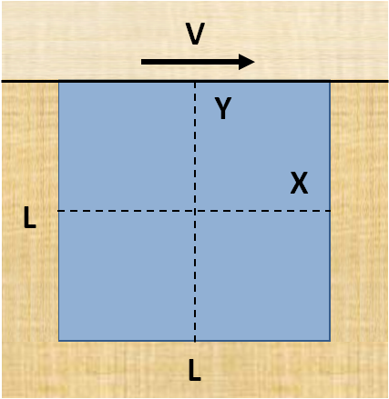
In this verification case, a square cavity with side length L=1 m is filled with fluid and the top wall (lid) moves at a constant speed of V = 1m/s. It was modeled as a 3-dimensional problem with 0.05 m thickness, considering periodic boundaries. The stationary walls and the moving lid are modeled with no-slip boundary condition. Laminar flow was evaluated for a Reynolds Re = 100.
The lid-driven cavity problem is illustrated in Figure 4.5: Lid-driven cavity validation case.. It is the same case presented in [7] and the reference results are compared for verification purposes.
The input parameters for the lid-driven cavity verification case setup are listed in Table 4.2: Lid-driven cavity case input parameters..
Table 4.2: Lid-driven cavity case input parameters.
| Parameter | Value | Unit |
|---|---|---|
|
Physical Model: | ||
| Thermal Model | Enabled |
- |
| Gravity (X) | 0 |  |
| Gravity (Y) | 0 |  |
| Gravity (Z) | 0 |  |
|
Wall Geometry: | ||
| Square Cavity Side (L) | 1.0 | m |
| Square Cavity Thickness | 0.05 | m |
| Lid Velocity (V) | 1.0 | m/s |
|
Fluid Properties: | ||
| Element size | 10 | mm |
| Initial Density | 10 |  |
| Dynamic Viscosity | 0.1 |  |
| Sound Speed | 10.0 | m/s |
| Boundary Type | No Slip Laminar | - |
| TurbulenceType | Laminar | - |
| Viscosity Type | Morris | - |
| Poission's Correction Type | None | - |
| Volumetric Inlet SPH Mass | 1.0 | kg |
|
Solver Parameters: | ||
|
Simulation Duration |
60 |
s |
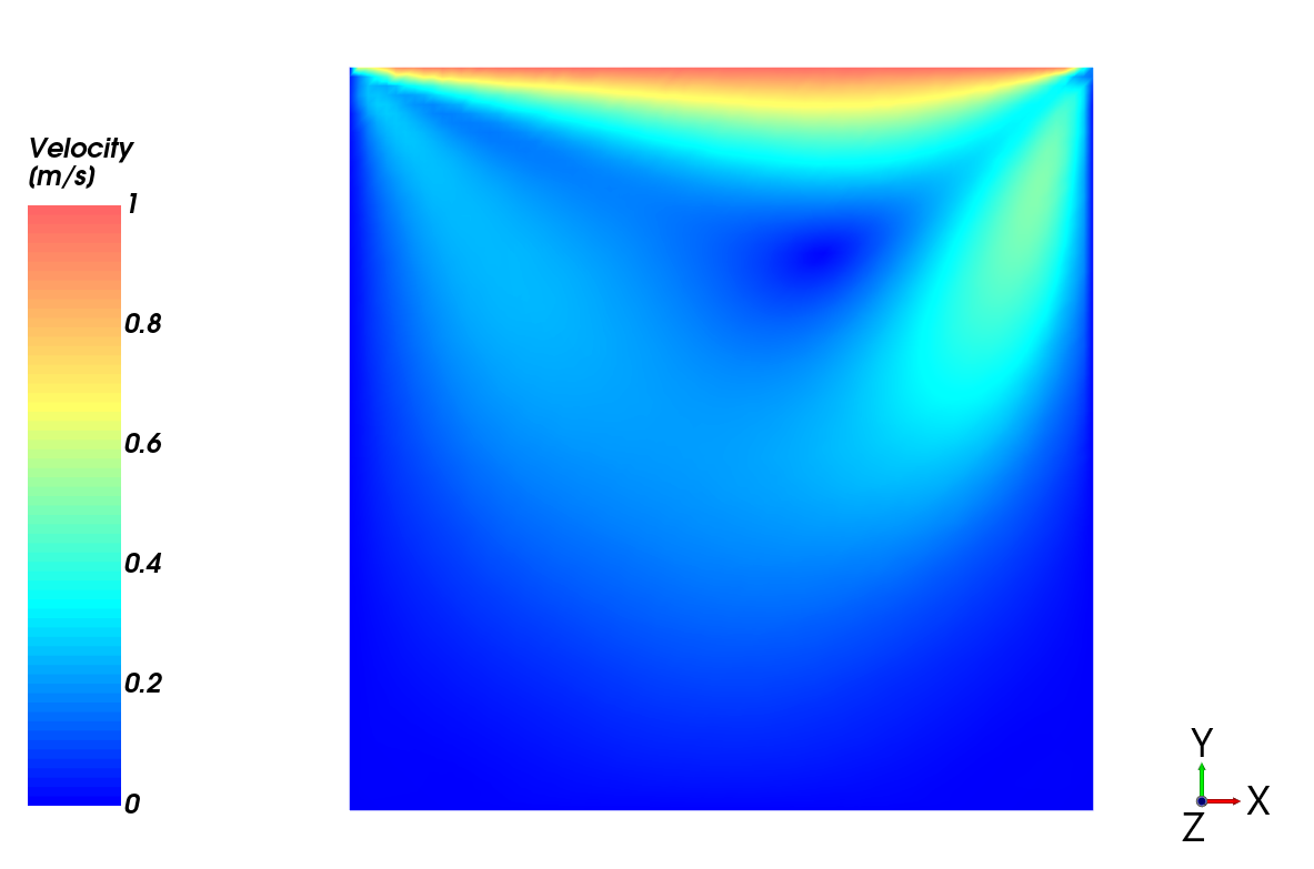
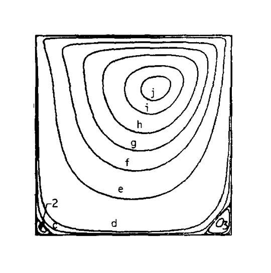
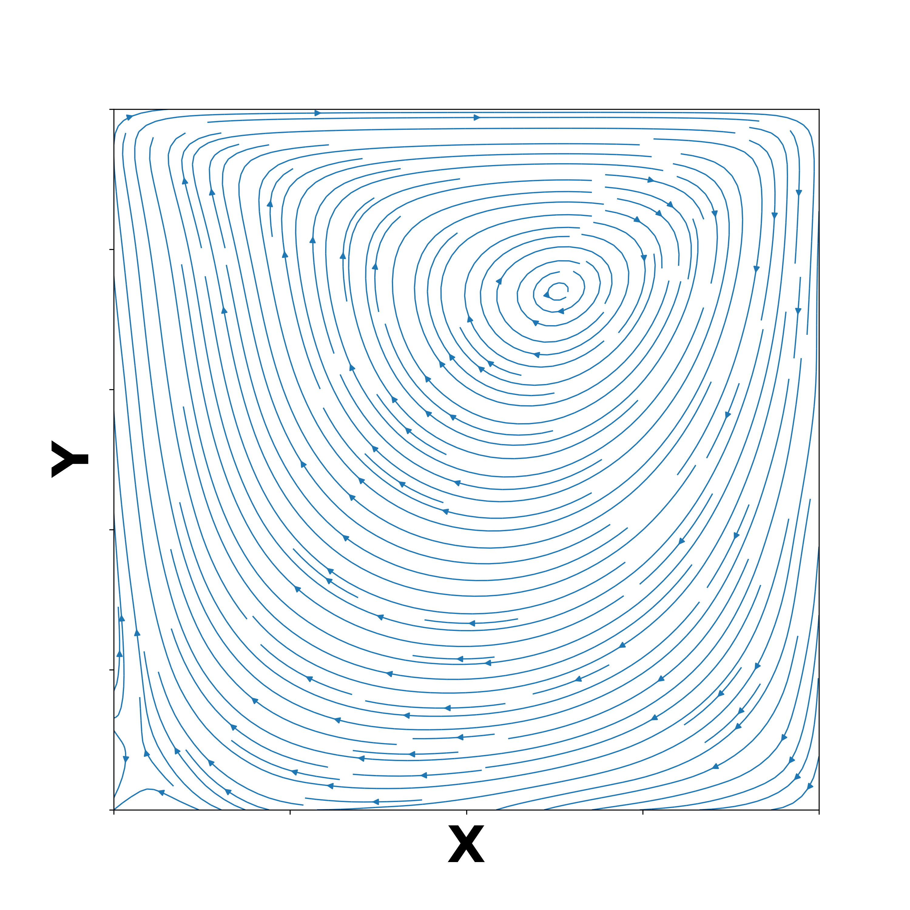
The velocity field of the fluid flow through the midplane on the z-direction of the cavity at Re=100 is shown in Figure 4.6: Velocity field through the cavity for Re=100., while Figure 4.7: Streamlines through the cavity for Re = 100: Ghia at alshows the streamline contours for the cavity flow on the same midplane. Figure 4.7: Streamlines through the cavity for Re = 100: Ghia at al(a) shows the streamlines obtained by [7], while Figure 4.7: Streamlines through the cavity for Re = 100: Ghia at al(b) shows the streamlines from the Rocky simulation.
A qualitative comparison can be done and one can see that the solutions present similar behavior. It is possible to observe that a vortex is generated by the shear force of the moving wall (lid) and the core of the vortex places at the upper half of the cavity.
Relevant verification parameters used in the literature for the lid-driven cavity problem are the horizontal fluid velocity (u) along the cavity vertical centerline, as well as the vertical fluid velocity (v) along the horizontal cavity centerline. Comparisons of the u and v fluid velocities along the lines through the cavity center for Re=100 are shown in Figure 4.9: Comparison of u-velocity along the vertical line through the cavity center for Re = 100. and Figure 4.10: Comparison of v-velocity along the horizontal line through the cavity center for Re=100., respectively. The fluid velocities calculated by Rocky presents strongly correlated values to the reference ones.
Figure 4.9: Comparison of u-velocity along the vertical line through the cavity center for Re = 100.
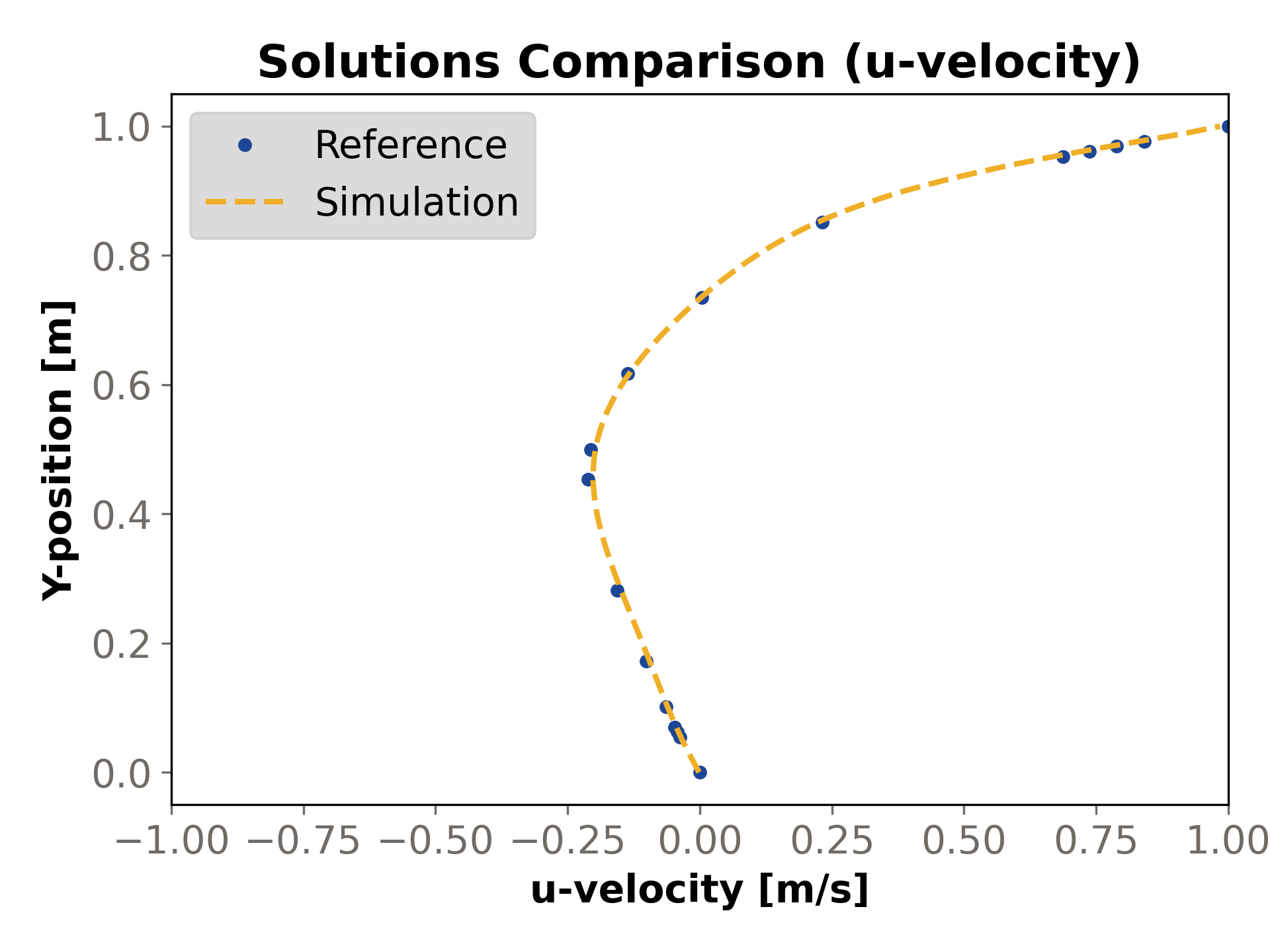
Figure 4.10: Comparison of v-velocity along the horizontal line through the cavity center for Re=100.
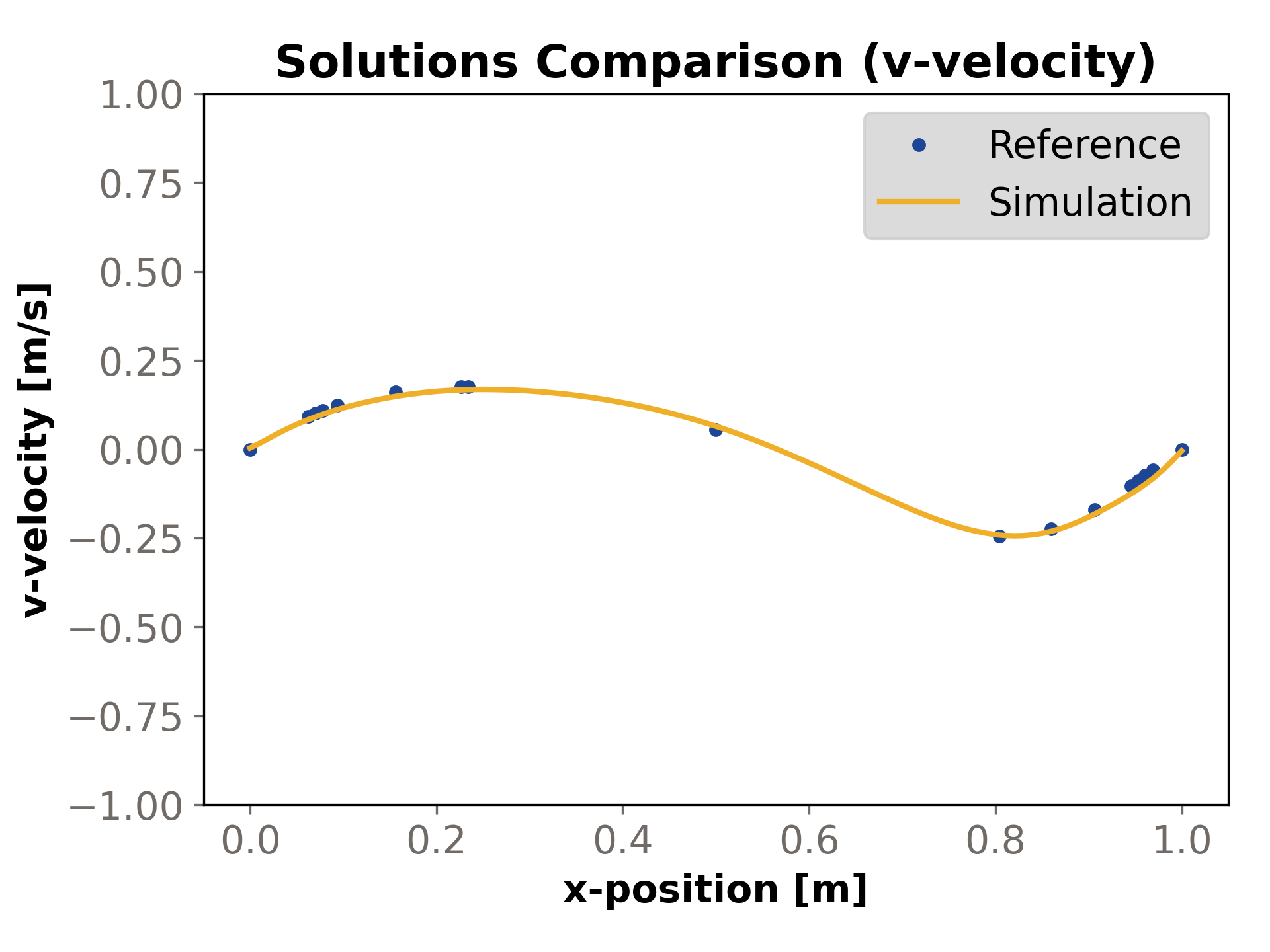
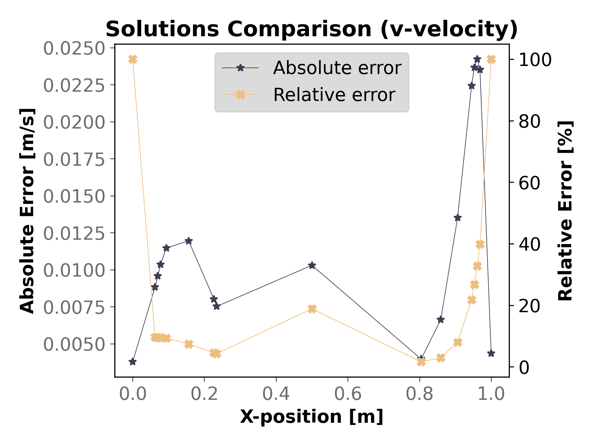
The comparisons of the absolute and relative errors between the velocities results for Re=100 are shown in Figure 4.11: Absolute and relative errors for u-velocity along the vertical line through the cavity center for Re = 100. and Figure 4.12: Absolute and relative errors v-velocity along the horizontal line through the cavity center for Re = 100.. The relative errors are mostly below 30% and higher differences can be observed at the points close to the stationary walls and other points where the velocities values are close to zero, in which high relative differences are expected.
Figure 4.11: Absolute and relative errors for u-velocity along the vertical line through the cavity center for Re = 100.
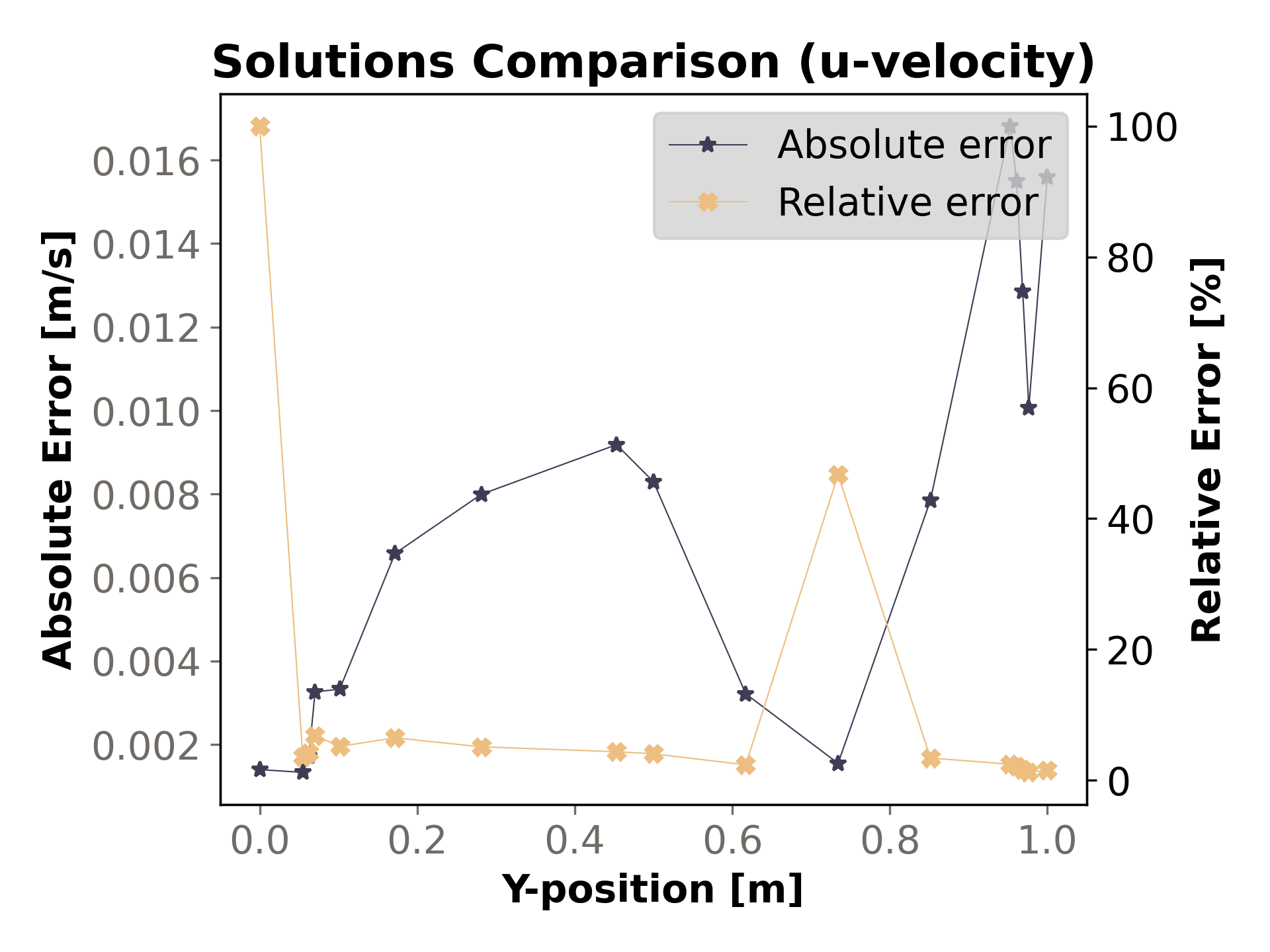
Figure 4.12: Absolute and relative errors v-velocity along the horizontal line through the cavity center for Re = 100.