Chapter 2: Parametric Analysis in Ansys Workbench Using Ansys Fluent

This tutorial is divided into the following sections:

2.1. Introduction

This tutorial illustrates using an Ansys Fluent fluid flow system in Ansys Workbench to set up and solve a three-dimensional turbulent fluid flow and heat transfer problem in an automotive heating, ventilation, and air conditioning (HVAC) duct system. Ansys Workbench uses parameters and design points to allow you to run optimization and what-if scenarios. You can define both input and output parameters in Ansys Fluent that can be used in your Ansys Workbench project. You can also define parameters in other applications including Ansys DesignModeler and Ansys CFD-Post. Once you have defined parameters for your system, a Parameters cell is added to the system and the Parameter Set bus bar is added to your project. This tutorial is designed to introduce you to the parametric analysis utility available in Ansys Workbench.

The tutorial starts with a Fluid Flow (Fluent) analysis system with pre-defined geometry and mesh components. Within this tutorial, you will redefine the geometry parameters created in Ansys DesignModeler by adding constraints to the input parameters. You will use Ansys Fluent to set up and solve the CFD problem. While defining the problem set-up, you will also learn to define input parameters in Ansys Fluent. The tutorial will also provide information on how to create output parameters in Ansys CFD-Post.

This tutorial demonstrates how to do the following:

Add constraints to the Ansys DesignModeler input parameters.
Create an Ansys Fluent fluid flow analysis system in Ansys Workbench.
Set up the CFD simulation in Ansys Fluent, which includes:
- Setting material properties and boundary conditions for a turbulent forced convection problem.
- Defining input parameters in Fluent
Define output parameters in CFD-Post
Create additional design points in Ansys Workbench.
Run multiple CFD simulations by updating the design points.
Analyze the results of each design point project in Ansys CFD-Post and Ansys Workbench.

Important: The mesh and solution settings for this tutorial are designed to demonstrate a basic parameterization simulation within a reasonable solution time-frame. Ordinarily, you would use additional mesh and solution settings to obtain a more accurate solution.

2.2. Prerequisites

This tutorial assumes that you are already familiar with the Ansys Workbench interface and its project workflow (for example, Ansys DesignModeler, Ansys Meshing, Ansys Fluent, and Ansys CFD-Post). This tutorial also assumes that you have completed the introductory Ansys Fluent tutorials, and that you are familiar with the Ansys Fluent graphical user interface. Some steps in the setup and solution procedure will not be shown explicitly.

2.3. Problem Description

In the past, evaluation of vehicle air conditioning systems was performed using prototypes and testing their performance in test labs. However, the design process of modern vehicle air conditioning (AC) systems improved with the introduction of Computer Aided Design (CAD), Computer Aided Engineering (CAE) and Computer Aided Manufacturing (CAM). The AC system specification will include minimum performance requirements, temperatures, control zones, flow rates, and so on. Performance testing using CFD may include fluid velocity (air flow), pressure values, and temperature distribution. Using CFD enables the analysis of fluid through very complex geometry and boundary conditions.

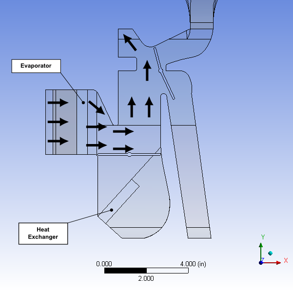
As part of the analysis, a designer can change the geometry of the system or the boundary conditions such as the inlet velocity, flow rate, and so on, and view the effect on fluid flow patterns. This tutorial illustrates the AC design process on a representative automotive HVAC system consisting of both an evaporator for cooling and a heat exchanger for heating requirements. This HVAC system is symmetric, so the geometry has been simplified using a plane of symmetry to reduce computation time.

Figure 2.1: Automotive HVAC System

Figure 2.2: HVAC System Valve Location Details

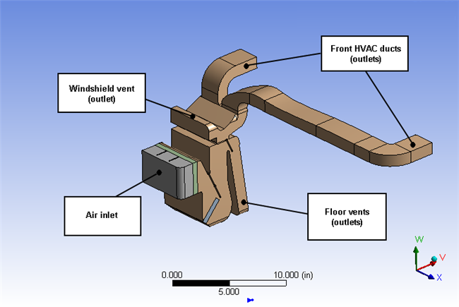
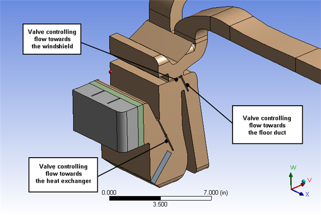
Figure 2.1: Automotive HVAC System shows a representative automotive HVAC system. The system has three valves (as shown in Figure 2.2: HVAC System Valve Location Details), which control the flow in the HVAC system. The three valves control:

Flow over the heat exchanger coils

Flow towards the duct controlling the flow through the floor vents

Flow towards the front vents or towards the windshield

Air enters the HVAC system at 310 K with a velocity of 0.5 m/sec through the air inlet and passes to the evaporator and then, depending on the position of the valve controlling flow to the heat exchanger, flows over or bypasses the heat exchanger. Depending on the cooling and heating requirements, either the evaporator or the heat exchanger would be operational, but not both at the same time. The position of the other two valves controls the flow towards the front panel, the windshield, or towards the floor ducts.

The motion of the valves is constrained. The valve controlling flow over the heat exchanger varies between 25° and 90°. The valve controlling the floor flow varies between 20° and 60°. The valve controlling flow towards front panel or windshield varies between 15° and 175°.

The evaporator load is about 200 W in the cooling cycle. The heat exchanger load is about 150 W.

This tutorial illustrates the easiest way to analyze the effects of the above parameters on the flow pattern/distribution and the outlet temperature of air (entering the passenger cabin). Using the parametric analysis capability in Ansys Workbench, a designer can check the performance of the system at various design points.

Figure 2.3: Flow Pattern for the Cooling Cycle

2.4. Setup and Solution

The following sections describe the setup and solution steps for this tutorial:

2.4.1. Preparation

To prepare for running this tutorial:

Download the workbench_parameter.zip file here .
Unzip the workbench_parameter.zip file to your working folder.
The extracted workbench_parameter folder contains a single archive file fluent-workbench-param.wbpz that includes all supporting input files of the starting Ansys Workbench project. The final result files incorporate Ansys Fluent and Ansys CFD-Post settings and all already defined design points (all that is required is to update the design points in the project to generate corresponding solutions).

2.4.2. Adding Constraints to Ansys DesignModeler Parameters in Ansys Workbench

In this step, you will start Ansys Workbench, open the project file, review existing parameters, create new parameters, and add constraints to existing Ansys DesignModeler parameters.

From the Windows Start menu, select Start > Ansys 2024 R2 > Workbench 2024 R2 to start Ansys Workbench.
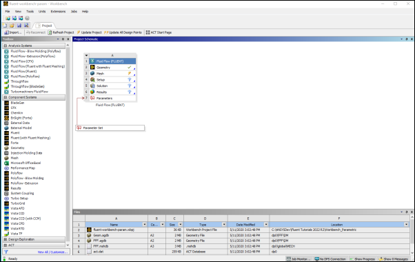
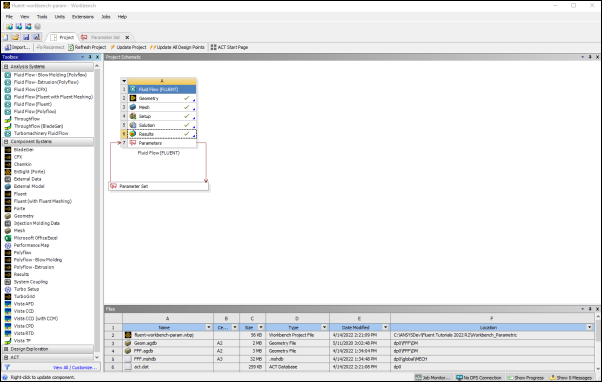
This displays the Ansys Workbench application window, which has the Toolbox on the left and the Project Schematic to its right. Various supported applications are listed in the Toolbox, and the components of the analysis system are displayed in the Project Schematic.
Note: When you first start Ansys Workbench, the Getting Started message window is displayed, offering assistance through the online help for using the application. You can keep the window open, or close it by clicking OK. If you need to access the online help at any time, use the Help menu, or press the F1 key.
Restore the archive of the starting Ansys Workbench project to your working directory.
File → Open...
Browse to your working directory, select the project archive file fluent-workbench-param.wbpz, and click Open.
Now that the project archive has been restored, the project will automatically open in Ansys Workbench.
Figure 2.4: The Project Loaded into Ansys Workbench

The project (fluent-workbench-param.wbpj) already has a Fluent-based fluid flow analysis system that includes the geometry and mesh, as well as some predefined parameters. You will first examine and edit parameters within Workbench, then later proceed to define the fluid flow model in Ansys Fluent.
Review the input parameters that have already been defined in Ansys DesignModeler.
1. Double-click the Parameter Set bus bar in the Ansys Workbench Project Schematic to open the Parameters Set tab.
  Note: To return to viewing the Project Schematic, click the Project tab.
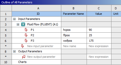
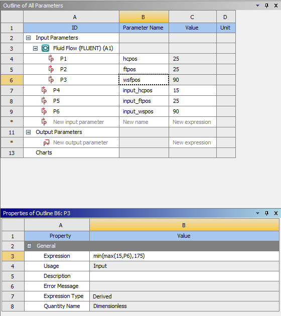
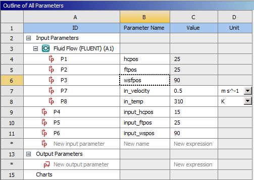
2. In the Outline of All Parameters view (Figure 2.5: Parameters Defined in Ansys DesignModeler), review the following existing parameters:
  - The parameter hcpos represents the valve position that controls the flow over the heat exchanger. When the valve is at an angle of 25°, it allows the flow to pass over the heat exchanger. When the angle is 90°, it completely blocks the flow towards the heat exchanger. Any value in between allows some flow to pass over the heat exchanger giving a mixed flow condition.
  - The parameter ftpos represents the valve position that controls flow towards the floor duct. When the valve is at an angle of 20°, it blocks the flow towards the floor duct and when the valve angle is 60°, it unblocks the flow.
  - The parameter wsfpos represents the valve position that controls flow towards the windshield and the front panel. When the valve is at an angle of 15°, it allows the entire flow to go towards the windshield. When the angle is 90°, it completely blocks the flow towards windshield as well as the front panel. When the angle is 175°, it allows the flow to go towards the windshield and the front panel.
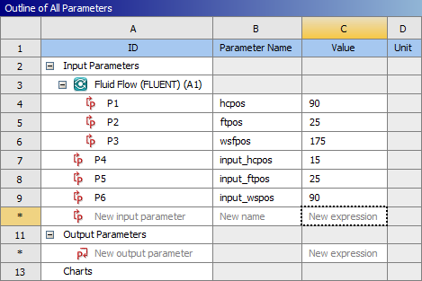
  Figure 2.5: Parameters Defined in Ansys DesignModeler
In the Outline of All Parameters view, create three new named input parameters.
1. In the row that contains New input parameter, click the parameter table cell with New name (under the Parameter Name column) and enter input_hcpos. Note the ID of the parameter that appears in column A of the table. For the new input parameter, the parameter ID is P4. In the Value column, enter 15.
2. In a similar manner, create two more parameters named input_ftpos and input_wsfpos. In the Value column, enter 25, and 90 for each new parameter (P5 and P6), respectively.
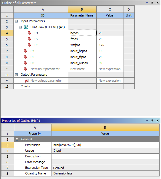
Figure 2.6: New Parameters Defined in Ansys Workbench
Select the row (or any cell in the row) that corresponds to the hcpos parameter. In the Properties of Outline view, change the value of the hcpos parameter in the Expression field from 90 to the expression min(max(25,P4),90). This puts a constraint on the value of hcpos, so that the value always remains between 25° and 90°. The redefined parameter hcpos is automatically passed to Ansys DesignModeler. Alternatively the same constraint can also be set using the expression max(25, min(P4,90)).
After defining this expression, the parameter becomes a derived parameter that is dependent on the value of the parameter input_hcpos with ID P4. The derived parameters are unavailable for editing in the Outline of All Parameters view and could be redefined only in the Properties of Outline view.
Important: When entering expressions, you must use the list and decimal delimiters associated with your selected language in the Workbench regional and language settings, which correspond to the regional settings on your machine. The instructions in this tutorial assume that your systems uses “.” as a decimal separator and “,” as a list separator.
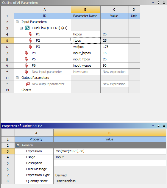
Figure 2.7: Constrained Parameter hcpos
Select the row or any cell in the row that corresponds to the ftpos parameter and create a similar expression for ftpos: min(max(20,P5),60).
Figure 2.8: Constrained Parameter ftpos
Create a similar expression for wsfpos: min(max(15,P6),175).
Figure 2.9: Constrained Parameter wsfpos
Click the X on the right side of the Parameters Set tab to close it and return to the Project Schematic.
Note the new status of the cells in the Fluid Flow (Fluent) analysis system. Since we have changed the values of hcpos, ftpos, and wsfpos to their new expressions, the Geometry and Mesh cells now indicates Refresh Required ( ).
Update the Geometry and Mesh cells.
1. Right-click the Geometry cell and select the Update option from the context menu.
2. Likewise, right-click the Mesh cell and select the Refresh option from the context menu. Once the cell is refreshed, then right-click the Mesh cell again and select the Update option from the context menu.
Save the project in Ansys Workbench.
In the main menu, select File → Save

2.4.3. Setting Up the CFD Simulation in Ansys Fluent

Now that you have edited the parameters for the project, you will set up a CFD analysis using Ansys Fluent. In this step, you will start Ansys Fluent, and begin setting up the CFD simulation.

2.4.3.1. Starting Ansys Fluent

In the Ansys Workbench Project Schematic, double-click the Setup cell in the Ansys Fluent fluid flow analysis system. You can also right-click the Setup cell to display the context menu where you can select the Edit... option.

When Ansys Fluent is first started, Fluent Launcher is displayed, allowing you to view and/or set certain Ansys Fluent start-up options.

Fluent Launcher allows you to decide which version of Ansys Fluent you will use, based on your geometry and on your processing capabilities.

Figure 2.10: Ansys Fluent Launcher

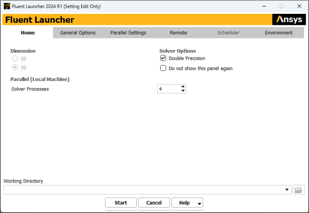
Ensure that the proper options are enabled.
Important: Note that the Dimension setting is already filled in and cannot be changed, since Ansys Fluent automatically sets it based on the mesh or geometry for the current system.
1. Ensure that the Double Precision option is enabled.
2. Set Solver Processes to 4 under Parallel (Local Machine).
Note: Fluent will retain your preferences for future sessions.
Click Start to launch Ansys Fluent.
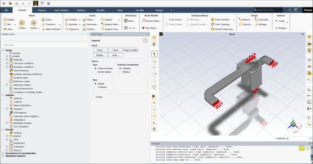
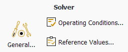
Figure 2.11: The Ansys Fluent Application

2.4.3.2. Setting Up Physics

In the Solver group of the Physics ribbon tab, retain the default selection of the steady pressure-based solver.
Physics → Solver
Set up your models for the CFD simulation using the Models group of the Physics ribbon tab.
1. Enable heat transfer by activating the energy equation.
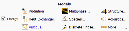
  In the Physics ribbon tab, enable Energy (Models group).
  Physics → Models → Energy
2. Enable the turbulence model.
  Physics → Models → Viscous...
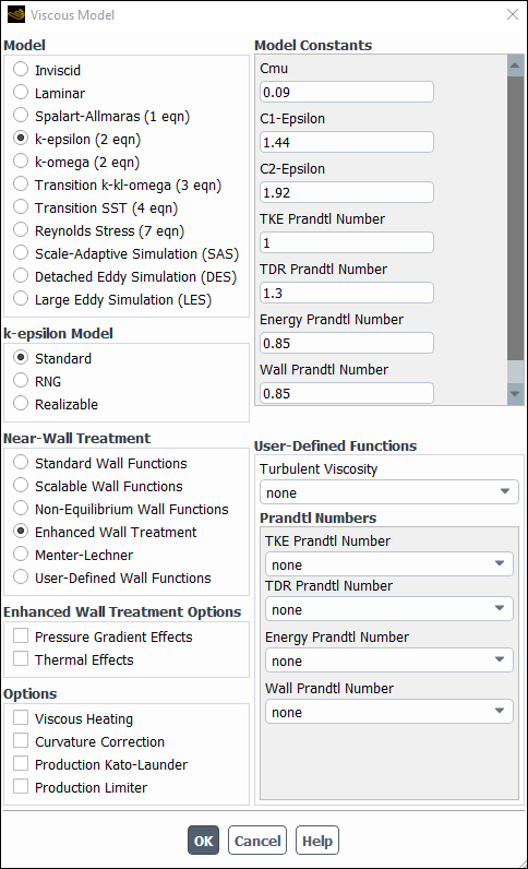
  1. Select the k-epsilon (2 eqn) from the Model group box.
  2. Select Enhanced Wall Treatment from the Near-Wall Treatment group box.
  3. Click OK to retain the other default settings and close the Viscous Model dialog box.
    Note that the Viscous... label in the ribbon is displayed in blue to indicate that the Viscous model is enabled.
Define a heat source cell zone condition for the evaporator volume.
Physics → Zones → Cell Zones
Note: All cell zones defined in your simulation are listed in the Cell Zone Conditions task page and under the Setup/Cell Zone Conditions tree branch.
1. In the Cell Zone Conditions task page, under the Zone list, select fluid-evaporator and click Edit... to open the Fluid dialog box.
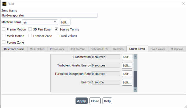
2. In the Fluid dialog box, enable Source Terms.
3. In the Source Terms tab, click the Edit... button next to Energy.
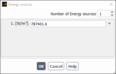
4. In the Energy sources dialog box, change the Number of Energy sources to 1.
5. For the new energy source, select constant from the drop-down list, and enter -787401.6 W/m³ — based on the evaporator load (200 W) divided by the evaporator volume (0.000254 m³) that was computed earlier.
6. Click OK to close the Energy sources dialog box.
7. Click Apply and close the Fluid dialog box.

2.4.4. Defining Input Parameters in Ansys Fluent

You have now started setting up the CFD analysis using Ansys Fluent. In this step, you will define boundary conditions and input parameters for the velocity inlet.

Define an input parameter called in_velocity for the velocity at the inlet boundary.
1. In the Physics tab, click Boundaries (Zones group).
  Physics → Zones → Boundaries
  This opens the Boundary Conditions task page.
  Note: All boundaries defined in the case are also displayed under the Setup/Boundary Conditions tree branch.
2. In the Boundary Conditions task page, click the Toggle Tree View button (in the upper right corner), and under the Group By category, select Zone Type. This displays boundary zones grouped by zone type.
3. Under the Inlet zone type, double-click inlet-air.
4. In the Velocity Inlet dialog box, from the Velocity Magnitude drop-down list, select New Input Parameter....
  This displays the Parameter Expression dialog box.
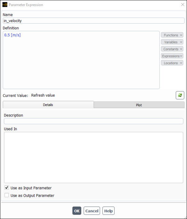
5. Enter in_velocity for the Name, and enter 0.5 [m s^-1] for Definition.
6. Click OK to close the Parameter Expression dialog box.
7. Under the Turbulence group box, from the Specification Method drop-down list, select Intensity and Hydraulic Diameter.
8. Retain the value of 5 for Turbulent Intensity.
9. Enter 0.061 for Hydraulic Diameter (m).
Define an input parameter called in_temp for the temperature at the inlet boundary.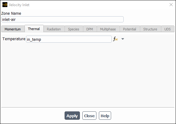
1. In the Thermal tab of the Velocity Inlet dialog box, select New Input Parameter... from the Temperature drop-down list.
2. Enter in_temp for the Name and enter 310 [K] for the Definition in the Parameter Expression dialog box.
3. Click OK to close the Parameter Expression dialog box.
4. Click Apply and Close the Velocity Inlet dialog box.
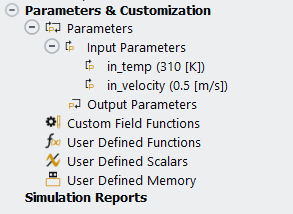
Review all of the input parameters that you have defined in Ansys Fluent under the Parameters & Customization/Parameters tree branch.
Parameters & Customization → Parameters → Input Parameters
Figure 2.12: The Input Parameters Sub-Branch in Ansys Fluent

These parameters are passed to Ansys Fluent component system in Ansys Workbench and are available for editing in Ansys Workbench (see Figure 2.13: The Parameters View in Ansys Workbench).

Figure 2.13: The Parameters View in Ansys Workbench
Set the turbulence parameters for backflow at the front outlets and foot outlets.
1. In the Boundary Conditions task page, type outlet in the Zone filter text entry field. Note that as you type, the names of the boundary zones beginning with the characters you entered appear in the boundary condition zone list.
  Note:
  The search string can include wildcards. For example, entering *let* will display all zone names containing let, such as inlet and outlet.
  To display all zones again, click the red X icon in the Zone filter.
2. Double-click outlet-front-mid.
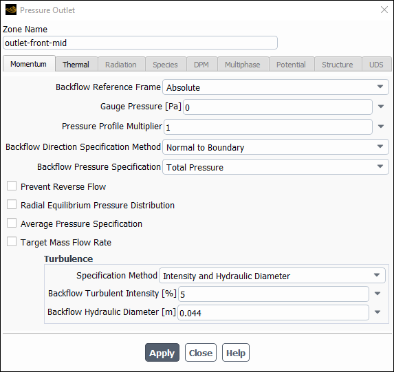
3. In the Pressure Outlet dialog box, under the Turbulence group box, select Intensity and Hydraulic Diameter from the Specification Method drop-down list.
4. Retain the value of 5 for Backflow Turbulent Intensity (%).
5. Enter 0.044 for Backflow Hydraulic Diameter (m).
  These values will only be used if reversed flow occurs at the outlets. It is a good idea to set reasonable values to prevent adverse convergence behavior if backflow occurs during the calculation.
6. Click Apply and Close the Pressure Outlet dialog box.
7. Copy the boundary conditions from outlet-front-mid to the other front outlet.
  Setup → Boundary Conditions → outlet-front-mid Copy...
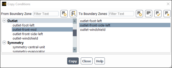
  1. Confirm that outlet-front-mid is selected in the From Boundary Zone selection list.
  2. Select outlet-front-side-left in the To Boundary Zones selection list.
  3. Click Copy to copy the boundary conditions.
    Fluent will display a dialog box asking you to confirm that you want to copy the boundary conditions.
  4. Click OK to confirm.
  5. Close the Copy Conditions dialog box.
8. In a similar manner, set the backflow turbulence conditions for outlet-foot-left using the values in the following table:
  Parameter Value
  Specification Method Intensity and Hydraulic Diameter
  Backflow Turbulent Intensity (%) 5
  Backflow Hydraulic Diameter (m) 0.052

Parameter	Value
Specification Method	Intensity and Hydraulic Diameter
Backflow Turbulent Intensity (%)	`5`
Backflow Hydraulic Diameter (m)	`0.052`

2.4.5. Solving

In the steps that follow, you will set up and run the calculation using the Solution ribbon tab.

Note: You can also use the task pages listed under the Solution branch in the tree to perform solution-related activities.

Set the Solution Methods.
Solution → Solution → Methods...
This will open the Solution Methods task page.
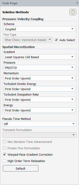
1. From the Scheme drop-down list, ensure that Coupled is selected.
2. In the Spatial Discretization group box, configure the following settings:
  
  Setting
  
  Value
  
  Pressure
  
  PRESTO!
  
  Momentum
  
  First Order Upwind
  
  Energy
  
  First Order Upwind
  
  This tutorial is primarily intended to demonstrate the use of parameterization and design points when running Fluent from Workbench. Therefore, you will run a simplified analysis using first order discretization, which will yield faster convergence. These settings were chosen to speed up solution time for this tutorial. Usually, for cases like this, we would recommend higher order discretization settings to be set for all flow equations to ensure improved results accuracy. The second-order scheme will provide a more accurate solution.
3. Ensure that Warped-Faced Gradient Correction is selected.
4. From the Pseudo Time Method ensure that Off is selected.
Initialize the flow field using the Initialization group of the Solution ribbon tab.
Solution → Initialization
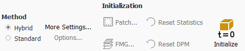
1. Retain the default selection of Hybrid Initialization.
2. Click the Initialize button.
Run the simulation in Ansys Fluent from the Run Calculation group of the Solution tab.
Solution → Run Calculation
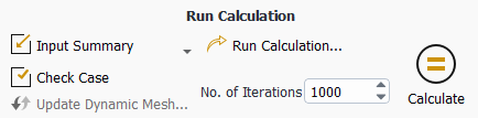
1. Enter 1000 for No. of Iterations
2. Click the Calculate button.
Throughout the calculation, Fluent displays a warning in the console regarding reversed flow at the outlets. This behavior is expected in this case since air is redirected to the outlets, creating small regions of recirculation.
Close Fluent.
File → Close Fluent
Save the project in Ansys Workbench.
File → Save

Setting	Value
Pressure	PRESTO!
Momentum	First Order Upwind
Energy	First Order Upwind

2.4.6. Postprocessing and Setting the Output Parameters in Ansys CFD-Post

In this step, you will visualize the results of your CFD simulation using Ansys CFD-Post. You will plot vectors that are colored by pressure, velocity, and temperature, on a plane within the geometry. In addition, you will create output parameters within Ansys CFD-Post for later use in Ansys Workbench.

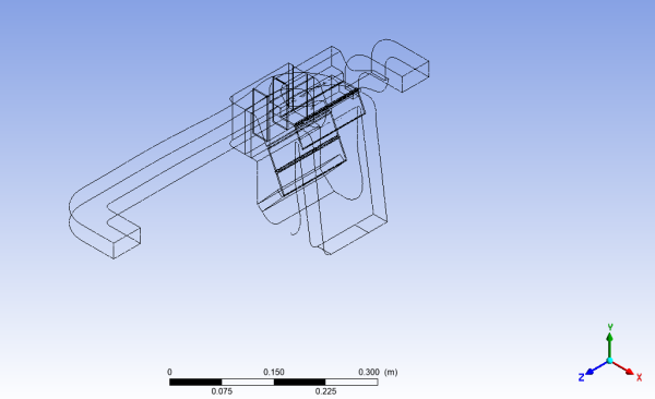
In the Ansys Workbench Project Schematic, double-click the Results cell in the Ansys Fluent fluid flow analysis system to start CFD-Post. You can also right-click the Results cell to display the context menu where you can select the Edit... option.

The CFD-Post application appears with the automotive HVAC geometry already loaded and displayed in outline mode. Note that Ansys Fluent results (that is, the case and data files) are also automatically loaded into CFD-Post.

Figure 2.14: The Automotive HVAC Geometry Loaded into CFD-Post

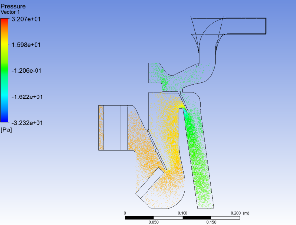
Plot vectors colored by pressure.
1. From the main menu, select Insert → Vector or click in the Ansys CFD-Post toolbar.
  This displays the Insert Vector dialog box.
2. Keep the default name of Vector 1 by clicking OK.
3. In the Details view for Vector 1, under the Geometry tab, configure the following settings.
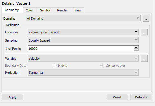
  1. Ensure All Domains is selected from the Domains drop-down list.
  2. From the Locations drop-down list, select symmetry central unit.
  3. From the Sampling drop-down list, select Equally Spaced.
  4. Set the # of Points to 10000.
  5. From the Projection drop-down list, select Tangential.
4. In the Color tab, configure the following settings.
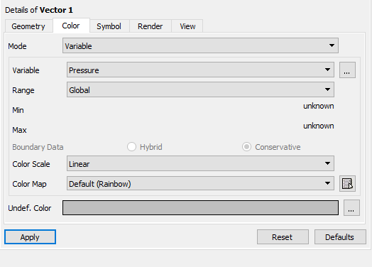
  1. From the Mode drop-down list, select Variable.
  2. From the Variable drop-down list, select Pressure.
5. In the Symbol tab, configure the following settings.
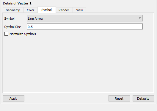
  1. Set the Symbol Size to 0.5.
6. Click Apply.
  Vector 1 appears under User Locations and Plots in the Outline tree view.
  In the graphics display window, note that symmetry-central-unit shows the vectors colored by pressure. Use the controls in CFD-Post to rotate the geometry (for example, clicking the dark blue axis in the axis triad of the graphics window). Zoom in to the view as shown in Figure 2.15: Vectors Colored by Pressure.
  Note: To better visualize the vector display, you can deselect the Wireframe view option under User Locations and Plots in the Outline tree view.
  Figure 2.15: Vectors Colored by Pressure
Plot vectors colored by velocity.
1. In the Details view for Vector 1, under the Color tab, configure the following settings.
  1. Select Velocity from the Variable drop-down list.
  2. Click Apply.
    The velocity vector plot appears on the symmetry-central-unit symmetry plane.
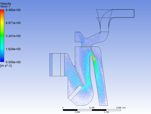
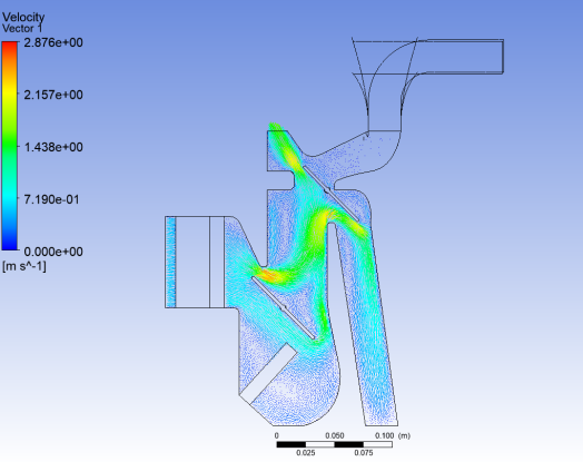
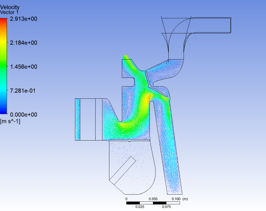
    Figure 2.16: Vectors Colored by Velocity
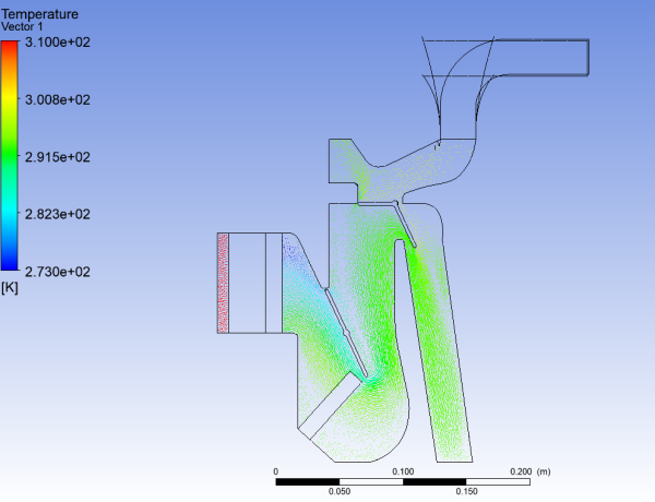
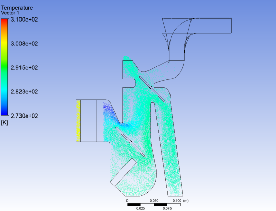
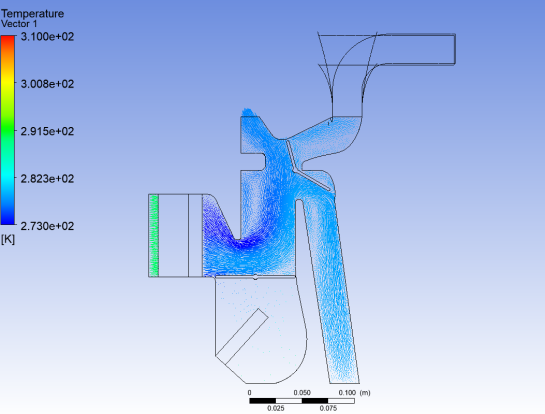
Plot vectors colored by temperature.
1. In the Details view for Vector 1, under the Color tab, configure the following settings.
  1. Select Temperature from the Variable drop-down list.
  2. Select User Specified from the Range drop-down list.
  3. Enter 273 K for the Min temperature value.
  4. Enter 310 K for the Max temperature value.
  5. Click Apply.
    The user-specified range is selected much narrower than the Global and Local ranges in order to better show the variation.
Figure 2.17: Vectors Colored by Temperature

Note the orientation of the various valves and how they impact the flow field. Later in this tutorial, you will change these valve angles to see how the flow field changes.
Create two surface groups.
Surface groups are collections of surface locations in CFD-Post. In this tutorial, two surface groups are created in CFD-Post that will represent all of the outlets and all of the front outlets. Once created, specific commands (or expressions) will be applied to these groups in order to calculate a particular numerical value at that surface.
1. Create a surface group consisting of all outlets.
  1. With the Outline tree view open in the CFD-Post tree view, open the Insert Surface Group dialog box.
    Insert → Location → Surface Group
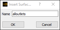
  2. Enter alloutlets for the Name of the surface group, and click OK to close the Insert Surface Group dialog box.
  3. In the Details view for the alloutlets surface group, in the Geometry tab, click the ellipsis icon next to Locations to display the Location Selector dialog box.
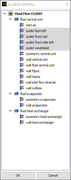
  4. Select all of the outlet surfaces (outlet foot left, outlet front mid, outlet front side left, and outlet windshield) in the Location Selector dialog box (hold Ctrl for multiple selection) and click OK.
  5. Click Apply in the Details view for the new surface group.
    alloutlets appears under User Locations and Plots in the Outline tree view.
2. Create a surface group for the front outlets.
  Perform the same steps as described above to create a surface group called frontoutlets with locations for the front outlets (outlet front mid and outlet front side left).
Create expressions in CFD-Post and mark them as Ansys Workbench output parameters.
In this tutorial, programmatic commands or expressions are written to obtain numerical values for the mass flow rate from all outlets, as well as at the front outlets, windshield, and foot outlets. The surface groups you defined earlier are used to write the expressions.
1. Create an expression for the mass flow from all outlets.
  1. With the Expressions tab open in the CFD-Post tree view, open the Insert Expression dialog box.
    Insert → Expression
  2. Enter floutfront for the Name of the expression and click OK to close the Insert Expression dialog box.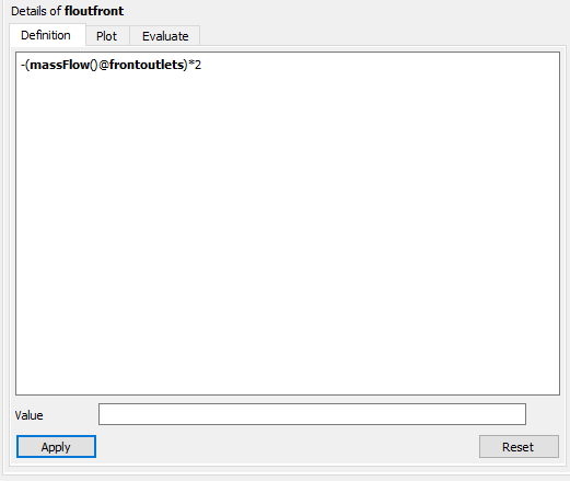
  3. In the Details view for the new expression, enter the following in the Definition tab.
    -(massFlow()@frontoutlets)*2
    
    The sign convention for massFlow() is such that a positive value represents flow into the domain and a negative value represents flow out of the domain. Since you are defining an expression for outflow from the ducts, you use the negative of the massFlow() result in the definition of the expression.
  4. Click Apply to obtain a Value for the expression.
    Note the new addition in the list of expressions in the Expressions tab in CFD-Post.
    In this case, there is a small net backflow into the front ducts.
  5. Right-click the new expression and select Use as Workbench Output Parameter from the context menu. A small “P” with a right-pointing arrow appears on the expression’s icon.
2. Create an expression for the mass flow from the wind shield.
  1. Perform the same steps as described above to create an expression called floutwindshield with the following definition:
    -(massFlow()@outlet windshield)*2
  2. Right-click the new expression and select Use as Workbench Output Parameter from the context menu.
3. Create an expression for the mass flow from the foot outlets.
  1. Perform the same steps as described above to create an expression called floutfoot with the following definition:
    -(massFlow()@outlet foot left)*2
  2. Right-click the new expression and select Use as Workbench Output Parameter from the context menu.
4. Create an expression for the mass weighted average outlet temperature.
  1. Perform the same steps as described above to create an expression called outlettemp with the following definition:
    massFlowAveAbs(Temperature)@alloutlets
  2. Right-click the new expression and select Use as Workbench Output Parameter from the context menu.
Close Ansys CFD-Post.
In the main menu, select File → Close CFD-POST to return to Ansys Workbench.
In the Outline of All Parameters view of the Parameter Set tab (double-click Parameter Set), review the newly-added output parameters that you specified in Ansys CFD-Post and when finished, click the Project tab to return to the Project Schematic.
If any of the cells in the analysis system require attention, update the project by clicking the Update Project button in the Ansys Workbench toolbar.
Optionally, review the list of files generated by Ansys Workbench. If the Files view is not open, select View → Files from the main menu.
You will notice additional files associated with the latest solution as well as those generated by CFD-Post.
Figure 2.18: The Updated Project Loaded into Ansys Workbench Displaying the Files View
Save the project in Ansys Workbench.
In the main menu, select File → Save
Note: You can also select the Save Project option from the CFD-Post File ribbon tab.

2.4.7. Creating Additional Design Points in Ansys Workbench

Parameters and design points are tools that allow you to analyze and explore a project by giving you the ability to run optimization and what-if scenarios. Design points are based on sets of parameter values. When you define input and output parameters in your Ansys Workbench project, you are essentially working with a design point. To perform optimization and what-if scenarios, you create multiple design points based on your original project. In this step, you will create additional design points for your project where you will be able to perform a comparison of your results by manipulating input parameters (such as the angles of the various valves within the automotive HVAC geometry). Ansys Workbench provides a Table of Design Points to make creating and manipulating design points more convenient.

Open the Table of Design Points.
1. In the Project Schematic, double-click the Parameter Set bus bar to open the Table of Design Points view. If the table is not visible, select Table from the View menu in Ansys Workbench.
  View → Table
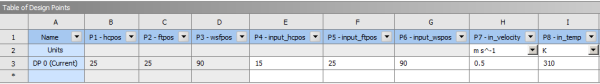
  The table of design points initially contains the current project as a design point (DP0), along with its corresponding input and output parameter values.
  Figure 2.19: Table of Design Points (with DP0)
  
  From this table, you can create new design points (or duplicate existing design points) and edit them (by varying one or more input parameters) to create separate analyses for future comparison of data.
Create a design point (DP1) by duplicating the current design point (DP0).
1. Right-click the Current design point and select Duplicate Design Point from the context menu.
  The cells autofill with the values from the Current row.
2. Scroll over to the far right to expose the Retain column in the table of design points, and ensure the check box in the row for the duplicated design point DP 1 (cell N4) is selected.
  This allows the data from this new design point to be saved before it is exported for future analysis.
Create another design point (DP2) by duplicating the DP1 design point.
1. Right-click the DP1 design point and select Duplicate Design Point from the context menu.
  Since this is a duplicate of DP1, this design point will also have its data retained.
Edit values for the input parameters for DP1 and DP2.
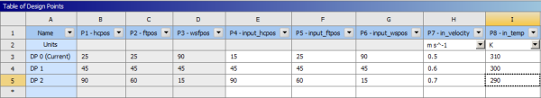
For DP1 and DP2, edit the values for your input parameters within the Table of Design Points as follows:
input_hcpos input_ftpos input_wsfpos in_velocity in_temp
DP1 45 45 45 0.6 300
DP2 90 60 15 0.7 290
Figure 2.20: Table of Design Points (with DP0, DP1, and DP2 Defined)

For demonstration purposes of this tutorial, in each design point, you are slightly changing the angles of each of the valves, and increasing the inlet velocity and decreasing the inlet temperature. Later, you will see how the results in each case vary.
Update all of your design points.
Click the Update all Design Points button in the Ansys Workbench toolbar. Alternatively, you can also select one or more design points, right-click, and select Update Selected Design Points from the context menu. Click OK to acknowledge the information message notifying you that some open editors may close during the update process. By updating the design points, Ansys Workbench takes the new values of the input parameters for each design point and updates the components of the associated system (for example, the geometry, mesh, settings, solution, and results), as well as any output parameters that have been defined.
Note: It may take significant time and/or computing resources to re-run the simulations for each design point.
Export the design points to separate projects.
This will allow you to work with calculated data for each design point.
1. Select the three design points, DP0, DP1, and DP2 (hold Shift for multiple selection).
2. Right-click the selected design points and select Export Selected Design Points.
  Note the addition of three more Ansys Workbench project files (and their corresponding folders) in your current working directory (fluent-workbench-param_dp0.wbpj, fluent-workbench-param_dp1.wbpj and fluent-workbench-param_dp2.wbpj). You can open each of these projects up separately and examine the results of each parameterized simulation.
Tip: You can easily access files in your project directory directly from the Files view by right-clicking any cell in the corresponding row and selecting Open Containing Folder from the menu that opens.
Inspect the output parameter values in Ansys Workbench.
Once all design points have been updated, you can use the table of design points to inspect the values of the output parameters you created in CFD-Post (for example, the mass flow parameters at the various outlets: floutfront, floutfoot, floutwindshield, and outlettemp). These, and the rest of the output parameters are listed to the far right in the table of design points.
Click the Project tab, located just above the Ansys Workbench toolbar, to return to the Project Schematic.
(Optional) View the list of files generated by Ansys Workbench.
View → Files
The additional files for the new design points are stored with their respective project files since you exported them.
Save the project in its current state in Ansys Workbench.
In the main menu, select File → Save.
Quit Ansys Workbench.
In the main menu, select File → Exit.

2.4.8. Postprocessing the New Design Points in CFD-Post

In this section, you will open the Ansys Workbench project for each of the design points and inspect the vector plots based on the new results of the simulations.

Study the results of the first design point (DP1).
1. Open the Ansys Workbench project for the first design point (DP1).
  In your current working folder, double-click the fluent-workbench-param_dp1.wbpj file to open Ansys Workbench.
2. Open CFD-Post by double-clicking the Results cell in the Project Schematic for the Fluid Flow (Fluent) analysis system.
3. View the vector plot colored by temperature. Ensure that Range in the Color tab is set to User Specified and the Min and Max temperature values are set to 273 K and 310 K, respectively.
  Figure 2.21: Vectors Colored by Temperature (DP1)
4. View the vector plot colored by pressure. Ensure that Range in the Color tab is set to Global.
  Figure 2.22: Vectors Colored by Pressure (DP1)
5. View the vector plot colored by velocity. Ensure that Range in the Color tab is set to Global.
  Figure 2.23: Vectors Colored by Velocity (DP1)
6. When you are finished viewing results of the design point DP1 in Ansys CFD-Post, select File → Close CFD-Post to quit Ansys CFD-Post and return to the Ansys Workbench Project Schematic, and then select File → Exit to exit from Ansys Workbench.
Study the results of the second design point (DP2).
1. Open the Ansys Workbench project for the second design point (DP2).
  In your current working folder, double-click the fluent-workbench-param_dp2.wbpj file to open Ansys Workbench.
2. Open CFD-Post by double-clicking the Results cell in the Project Schematic for the Fluid Flow (Fluent) analysis system.
3. View the vector plot colored by temperature. Ensure that Range in the Color tab is set to User Specified and the Min and Max temperature values are set and the Min and Max temperature values are set to 273 K and 310 K, respectively.
  Figure 2.24: Vectors Colored by Temperature (DP2)
4. View the vector plot colored by pressure. Ensure that Range in the Color tab is set to Global.
  Figure 2.25: Vectors Colored by Pressure (DP2)
5. View the vector plot colored by velocity. Ensure that Range in the Color tab is set to Global.
  Figure 2.26: Vectors Colored by Velocity (DP2)
When you are finished viewing results in Ansys CFD-Post, select File → Close CFD-Post to quit Ansys CFD-Post and return to the Ansys Workbench Project Schematic, and then select File → Exit to exit from Ansys Workbench.

2.4.9. Summary

In this tutorial, input and output parameters were created within Ansys Workbench, Ansys Fluent, and Ansys CFD-Post in order to study the airflow in an automotive HVAC system. Ansys Fluent was used to calculate the fluid flow throughout the geometry using the computational mesh, and Ansys CFD-Post was used to analyze the results. Ansys Workbench was used to create additional design points based on the original settings, and the corresponding simulations were run to create separate projects where parameterized analysis could be performed to study the effects of variable angles of the inlet valves, velocities, and temperatures. Also, note that simplified solution settings were used in this tutorial to speed up the solution time. For more improved solution accuracy, you would typically use denser mesh and higher order discretization for all flow equations.

	`input_hcpos`	`input_ftpos`	`input_wsfpos`	`in_velocity`	`in_temp`
DP1	45	45	45	0.6	300
DP2	90	60	15	0.7	290