


The momentum source terms added to the fluid momentum equation can model the bulk behavior of the fluid flow around the rigid solid object. However, they do not track the immersed solid boundary accurately, or provide any sort of wall treatment near the immersed solid boundary to account for the boundary layer, or other effects on the flow. In order to better resolve these boundary effects, CFX-Solver imposes a modified forcing term near the immersed boundary
This section describes notation used in the following sections pertaining to immersed solids.
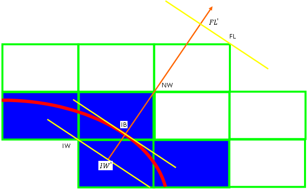
Figure 1.3: Notation for Nodes Near the Immersed Solid Boundary shows a schematic diagram of an immersed solid boundary (shown as a red line). The nodes and points near the boundary are labeled for reference in the following sections. The meaning of each label is tabulated below.
|
Label |
Meaning |
|---|---|
|
IW |
in-wall node |
|
IW′ |
in-wall point |
|
NW |
near-wall node |
|
IB |
point on the immersed solid boundary |
|
FL |
fluid node |
|
FL′ |
fluid point |
In the figure, the orange arrow represents the wall normal direction corresponding to the given NW node. For each NW node, the solver searches through the surrounding fluid nodes, and determines the corresponding FL node using a procedure that takes into account the normal distance from the immersed boundary and the deviation from the normal direction.
Other notes about notation:
"NIBG" elements are elements between corresponding NW and IW nodes. These are elements that the immersed solid surface cuts through, and are colored blue in the figure above.
"NIBF" elements are elements between corresponding FL and NW nodes. These are elements that are immediately adjacent to the "NIBG" elements and are colored white in the figure above.
 is the wall distance between the NW node and the
IB point along the wall normal direction.
is the wall distance between the NW node and the
IB point along the wall normal direction. is the wall distance between the NW node and the
IW′ point.
is the wall distance between the NW node and the
IW′ point. is the wall distance between the FL′ point and the NW node.
For laminar flows, no wall scale equation is solved. Instead, the velocity near the immersed boundary is computed based on the wall distance, assuming constant wall shear in the boundary profile region.
The tangential forcing velocity at the near-wall fluid nodes is governed by:
 | (1–136) |
where  is the tangential forcing velocity at the NW node,
 is the dynamic
viscosity at the NW node,
is the dynamic
viscosity at the NW node,  and
and  are, respectively, the fluid velocity and dynamic viscosity at
the FL node, and
are, respectively, the fluid velocity and dynamic viscosity at
the FL node, and  is the distance between the corresponding
FL′ point and NW node. Note that
is the distance between the corresponding
FL′ point and NW node. Note that  is essentially the normal distance
between this node and the immersed boundary.
is essentially the normal distance
between this node and the immersed boundary.
The normal forcing velocity at the NW node is computed as the normal component of the velocity at the IB point on the immersed boundary:
 | (1–137) |
The fluid velocity at the near-wall nodes is forced to be:
 | (1–138) |
In this way, the velocity field is forced to flow around the immersed boundary to avoid (or alleviate) the problem of streamlines penetrating the immersed solid.
For moving immersed solids or high Reynolds number turbulence cases, it is usually not possible to generate a fine mesh that resolves the laminar sub-layer. Hence, wall functions are used for fluid elements near the immersed boundary. The implementation of wall functions for immersed solids is more complicated than for wall functions near regular walls because of the non-uniform wall distance for elements next to the immersed boundary.
For fluid nodes that are inside the immersed solid, the wall distance is set to zero. For fluid nodes near the immersed solid, the wall distance is computed as a function of the wall scales. The wall scales are set algebraically to zero for fluid nodes inside the immersed solid, but the shape of the immersed boundary is not properly taken into account for the wall scale equation.
For the near-immersed-boundary nodes, the physical distance from the immersed boundary tracking method is used to implement the turbulent wall functions.
The wall distance from the modified wall scale equation is used to compute the two blending factors. The production and dissipation terms inside the immersed solid are reset to zero for both the turbulent kinetic energy equation and turbulent frequency equation. This way, the turbulent kinetic energy and turbulent frequency will be solved without any source terms and solutions will serve as a natural condition for the fluid turbulence equations.
In the SST turbulence model, the turbulent eddy viscosity is computed from the turbulent kinetic energy and turbulent frequency:
 | (1–139) |
In general, it is impractical (if not impossible) to have a
mesh which resolves the sublayer, and therefore, it is necessary to
specify  taking account
of the logarithmic region.
taking account
of the logarithmic region.
 | (1–140) |
 | (1–141) |
 | (1–142) |
 | (1–143) |
 | (1–144) |
Here,  is the fluid tangential
velocity relative to the immersed boundary, and
is the fluid tangential
velocity relative to the immersed boundary, and  is computed as the distance from the near-immersed-solid nodes to
the immersed boundary. In the scalable wall function, the lower value
of
is computed as the distance from the near-immersed-solid nodes to
the immersed boundary. In the scalable wall function, the lower value
of  is limited to 11.06 at the intersection
between the logarithmic and the linear near wall profile.
is limited to 11.06 at the intersection
between the logarithmic and the linear near wall profile.
Further, the velocity at the NW nodes is forced according to the wall function:
 | (1–145) |
Similar to the case of laminar flow, the tangential velocity on the NW nodes is enforced according to equation Equation 1–145 and the momentum source term is computed taking into account both the wall normal velocity and tangential forcing velocity:
 | (1–146) |
In this way, the velocity field will be forced to flow around the immersed boundary to avoid (or alleviate) the problem of streamlines penetrating the immersed solid.