Chapter 8: Modeling Transient Compressible Flow

This tutorial is divided into the following sections:

8.1. Introduction

In this tutorial, Ansys Fluent’s density-based implicit solver is used to predict the time-dependent flow through a two-dimensional nozzle. As an initial condition for the transient problem, a steady-state solution is generated to provide the initial values for the mass flow rate at the nozzle exit.

This tutorial demonstrates how to do the following:

Calculate a steady-state solution (using the density-based implicit solver) as an initial condition for a transient flow prediction.
Define a transient boundary condition using an expression.
Use automatic mesh adaption for both steady-state and transient flows.
Calculate a transient solution using the second-order implicit transient formulation and the density-based implicit solver.

8.2. Prerequisites

This tutorial is written with the assumption that you have completed the introductory tutorials found in this manual and that you are familiar with the Ansys Fluent outline view and ribbon structure. Some steps in the setup and solution procedure will not be shown explicitly.

8.3. Problem Description

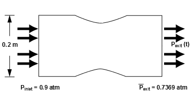
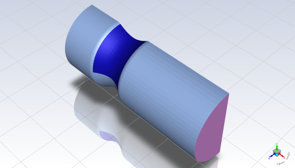
The geometry to be considered in this tutorial is shown in Figure 8.1: Problem Specification. Flow through a simple nozzle is simulated as a 3D model. The nozzle has an inlet height of 0.2 m, and the nozzle contours have a sinusoidal shape that produces a 20% reduction in flow area. Symmetry allows only half of the nozzle to be modeled.

Figure 8.1: Problem Specification

8.4. Setup and Solution

The following sections describe the setup and solution steps for this tutorial:

8.4.1. Preparation

To prepare for running this tutorial:

Download the transient_compressible.zip file here .
Unzip transient_compressible.zip to your working directory.
The geometry file nozzle.scdoc can be found in the folder.
Use the Fluent Launcher to start Ansys Fluent.
Select Meshing in the top-left selection list to start Fluent in Meshing Mode.
Select 3D under Dimension.
Disable Double Precision under Options.
Set Meshing Processes and Solver Processes to 4 under Parallel (Local Machine).

8.4.2. Meshing Workflow

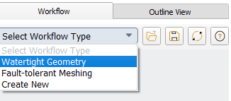
Start the meshing workflow.
1. In the Workflow tab, select the Watertight Geometry workflow.
2. Review the tasks of the workflow.
  
  Each task is designated with an icon indicating its state (for example, as complete, incomplete, etc. For more information, see Understanding Task States in the Fluent User's Guide). All tasks are initially incomplete and you proceed through the workflow completing all tasks. Additional tasks are also available for the workflow. For more information, see Customizing Workflows in the Fluent User's Guide.
Import the CAD geometry (nozzle.scdoc).
1. Select the Import Geometry task.
2. For Units, select mm.
3. For File Name, enter the path and file name for the CAD geometry that you want to import (nozzle.scdoc).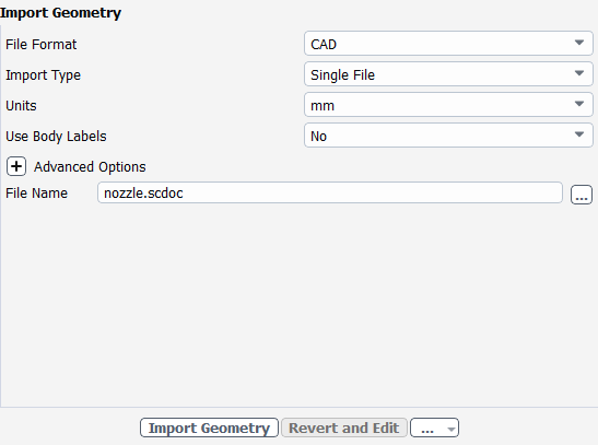
  
  Note: The workflow only supports *.scdoc (SpaceClaim), Workbench (.agdb), and the intermediary *.pmdb file formats.
4. Click Import Geometry.
  This will update the task, display the geometry in the graphics window and allow you to proceed onto the next task in the workflow.
  Figure 8.2: The Imported CAD Geometry for the Nozzle
  
  Note: Alternatively, the ... button next to File Name can be used to locate the CAD geometry file, after which, the Import Geometry task automatically updates, displaying the geometry in the graphics window, and the workflow automatically progresses to the next task.
  Throughout the workflow, you are able to return to a task and change its settings using either the Edit button, or the Revert and Edit button.
In the Add Local Sizing task, retain the default no and click Update to complete this task and proceed to the next task in the workflow.
Generate the surface mesh.
With the local sizing set as described above, the global surface mesh sizing only defines the largest elements on other surfaces.
1. In the Generate the Surface Mesh task, you can set various properties of the surface mesh for the faceted geometry.
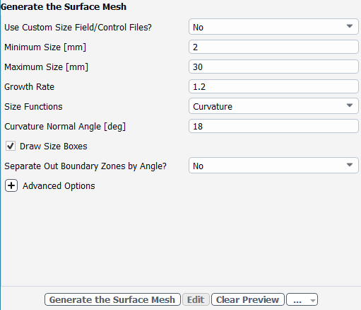
2. Specify 2 for the Minimum Size.
3. Specify 30 for the Maximum Size.
  Note: The red boxes displayed on the geometry in the graphics window are a graphical representation of size settings. These boxes change size as the values change, and they can be hidden by using the Clear Preview button.
4. Specify 1.2 for the Growth Rate.
5. Select Curvature option under Size Functions.
6. Specify 18 for the Curvature Normal Angle.
7. Click Generate the Surface Mesh to complete this task and proceed to the next task in the workflow.
Describe the geometry.
When you select the Describe Geometry task, you are prompted with questions relating to the nature of the imported geometry.
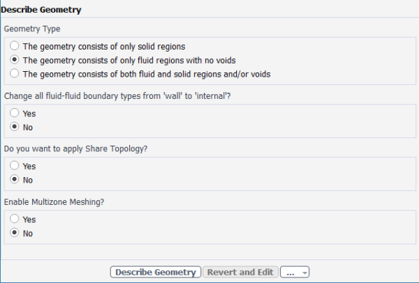
1. Select The geometry consists of only fluid regions with no voids option under Geometry Type, since this model contains only the fluid region.
2. Keep the rest of the default settings for this task.
3. Click Describe Geometry to complete this task and proceed to the next task in the workflow.
Confirm and update the boundaries.
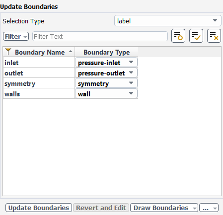
1. Select the Update Boundaries task, where you can inspect the mesh boundaries and confirm and change any designated boundaries accordingly. Ansys Fluent attempts to determine the correct arrangement of boundaries automatically.
2. Select pressure-inlet for the inlet boundary type.
3. Click Update Boundaries and proceed to the next task.
Update your regions.
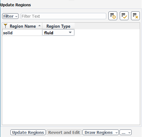
1. Select the Update Regions task, where you can review and change the tabulated names and types of the various regions that have been generated from your imported geometry and change them as needed.
2. The proposed region type is correct, so click Update Regions to update your settings.
Add boundary layers.
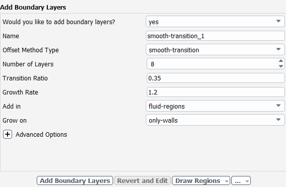
1. Select the Add Boundary Layers task, where you can set properties of the boundary layer mesh.
  For the Add Boundary Layers task, ensure yes is selected at the prompt as to define boundary layer settings. In this task, you can define specific details for capturing the boundary layer in and around your geometry.
2. Specify 8 for the Number of Layers.
3. Specify 0.35 for the Transition Ratio.
4. Click Add Boundary Layers.
Generating the volume mesh.
With the local sizing set as described above, including bodies of influence, the global volume mesh sizing only defines the largest elements in the flow domain. In this case, the maximum is set to be consistent with the specified global surface mesh sizing.
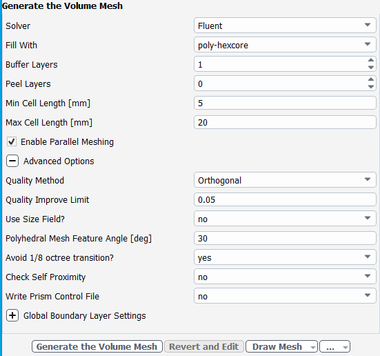
1. Select the Generate the Volume Mesh task, to set properties of the volume mesh.
2. Select the poly-hexcore for Fill With.
3. Specify 1 for Buffer Layers.
4. Specify 0 for Peel Layers.
5. Specify 5 for the Min Cell Length.
6. Specify 20 for the Max Cell Length.
  Note: The red boxes displayed on the geometry in the graphics window are a graphical representation of size settings. These boxes change size as the values change, and they can be hidden by using the Clear Preview button.
7. Expand the Advanced Options task, to set properties of the volume mesh.
8. Specify yes for Avoid 1/8 octree transtion?.
9. Click Generate the Volume Mesh.
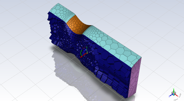
  Ansys Fluent will apply your settings and proceed to generate a volume mesh for the geometry.. The mesh is displayed in the graphics window and a clipping plane is automatically inserted with a layer of cells drawn so that you can quickly see the details of the volume mesh.
Check the mesh.
Mesh → Check → Perform Mesh Check
Save the mesh file (nozzle.msh.h5).
File → Write → Mesh...
Switch to Solution mode.
Now that a mesh has been generated using Ansys Fluent in meshing mode, you can now switch to solver mode to complete the set up of the simulation. Note that to obtain more accurate solutions a higher quality mesh should be used.
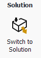
We have just checked the mesh, so select Yes when prompted to switch to solution mode.

8.4.3. Set Units

For convenience, change the unit of measurement for pressure.
The pressure for this problem is specified in atm, which is not the default unit in Ansys Fluent. You must redefine the pressure unit as atm.
Domain → Mesh → Units...
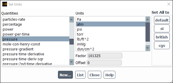
1. Select pressure in the Quantities selection list.
  Scroll down the list to find pressure.
2. Select atm in the Units selection list.
3. Close the Set Units dialog box.

8.4.4. Solution

Select the solver settings.
Setup → General → Density-Based
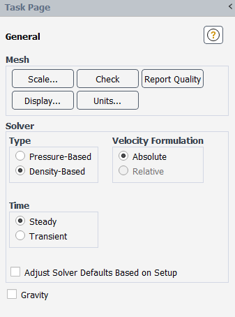
1. Select Density-Based in the General task page (Solver group box, under Type).
  The density-based implicit solver is the solver of choice for compressible, transonic flows without significant regions of low-speed flow. In cases with significant low-speed flow regions, the pressure-based solver is preferred. Also, for transient cases with traveling shocks, the density-based explicit solver with explicit time stepping may be the most efficient.
2. Retain the default selection of Steady from the Time list.
  Note: You will solve for the steady flow through the nozzle initially. In later steps, you will use these initial results as a starting point for a transient calculation.

8.4.5. Models

Enable the energy equation.
Physics → Models → Energy
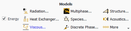
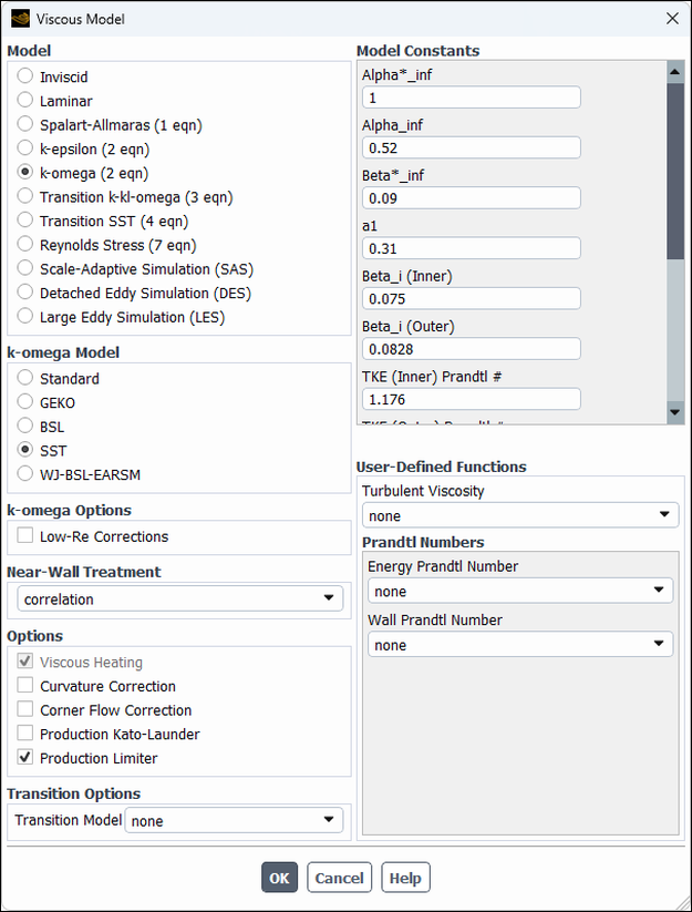
Retain the default k-omega SST turbulence model.
Physics → Models → Viscous...

8.4.6. Materials

Define the settings for air, the default fluid material.
Setup → Materials → Fluid → air Edit...
1. Select ideal-gas from the Density drop-down list in the Properties group box, so that the ideal gas law is used to calculate density.
  Note: Ansys Fluent automatically enables the solution of the energy equation when the ideal gas law is used, in case you did not already enable it manually in the Energy dialog box.
2. Retain the default values for all other properties.
3. Click the Change/Create button to save your change.
4. Close the Create/Edit Materials dialog box.

8.4.7. Operating Conditions

Define the operating pressure.
Physics → Solver → Operating Conditions...
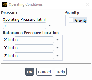
1. Enter 0 atm for Operating Pressure.
2. Click OK to close the Operating Conditions dialog box.
Since you have set the operating pressure to zero, you will specify the boundary condition inputs for pressure in terms of absolute pressures when you define them in the next step. Boundary condition inputs for pressure should always be relative to the value used for operating pressure.

8.4.8. Boundary Conditions

Define the boundary conditions for the nozzle inlet.
Setup → Boundary Conditions → Inlet → inlet (pressure-inlet) Edit...
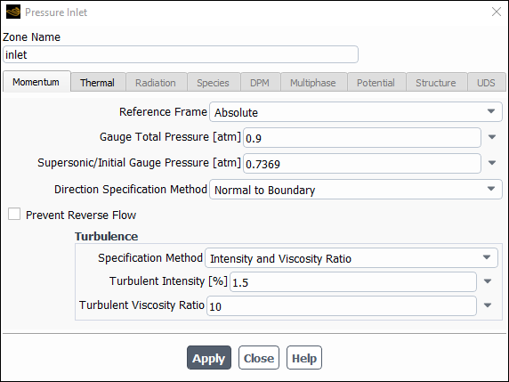
1. Enter 0.9 atm for Gauge Total Pressure.
2. Enter 0.7369 atm for Supersonic/Initial Gauge Pressure.
  The inlet static pressure estimate is the mean pressure at the nozzle exit. This value will be used during the solution initialization phase to provide a guess for the nozzle velocity.
3. Retain Intensity and Viscosity Ratio from the Specification Method drop-down list in the Turbulence group box.
4. Enter 1.5% for Turbulent Intensity.
5. Retain the setting of 10 for Turbulent Viscosity Ratio.
6. Click Apply and close the Pressure Inlet dialog box.
Define the boundary conditions for the nozzle exit.
Setup → Boundary Conditions → Outlet → outlet (pressure-outlet) Edit...
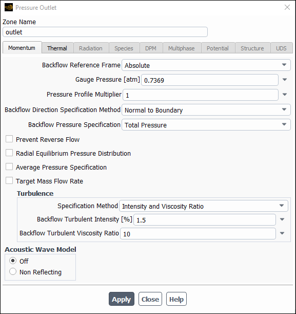
1. Enter 0.7369 atm for Gauge Pressure.
2. Retain Intensity and Viscosity Ratio from the Specification Method drop-down list in the Turbulence group box.
3. Enter 1.5% for Backflow Turbulent Intensity.
4. Retain the setting of 10 for Backflow Turbulent Viscosity Ratio.
  If substantial backflow occurs at the outlet, you may need to adjust the backflow values to levels close to the actual exit conditions.
5. Click Apply and close the Pressure Outlet dialog box.

8.4.9. Solution: Steady Flow

In this step, you will generate a steady-state flow solution that will be used as an initial condition for the time-dependent solution.

Define the solution parameters.
Solution → Solution → Methods...
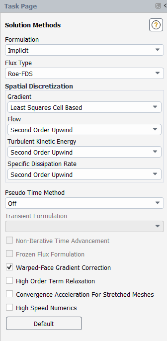
1. Retain the default selection of Least Squares Cell Based from the Gradient drop-down list in the Spatial Discretization group box.
Modify the Courant Number.
Solution → Controls → Controls...
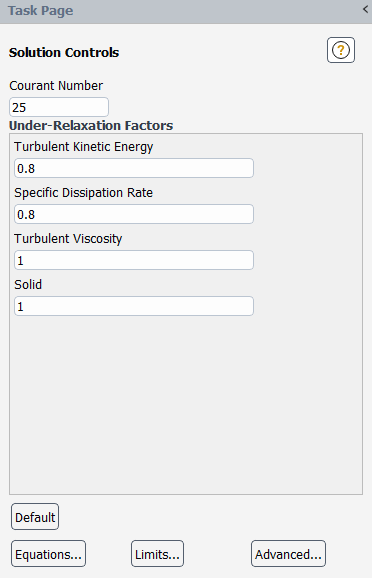
1. Enter 25 for the Courant Number.
  Note: The default Courant number for the density-based implicit formulation is 5. For relatively simple problems, setting the Courant number to 10, 20, 100, or even higher value may be suitable and produce fast and stable convergence. However, if you encounter convergence difficulties at the startup of the simulation of a properly set up problem, then you should consider setting the Courant number to its default value of 5. As the solution progresses, you can start to gradually increase the Courant number until the final convergence is reached.
2. Retain the default values for the Under-Relaxation Factors.
Enable the plotting of residuals.
Solution → Reports → Residuals...
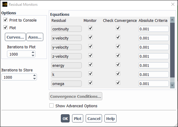
1. Ensure that Plot is enabled in the Options group box.
2. Click OK to close the Residual Monitors dialog box.
Create the surface report definition for mass flow rate at the flow exit.
Solution → Reports → Definitions → New → Surface Report → Mass Flow Rate...
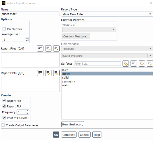
1. Enter outlet-mdot for Name.
2. Select outlet in the Surfaces selection list.
3. In the Create group box, enable Report File, Report Plot and Print to Console.
  Note: When Report File is enabled in the Surface Report Definition dialog box, the mass flow rate history will be written to a file. If you do not enable this option, the history information will be lost when you exit Ansys Fluent.
4. Click OK to close the Surface Report Definition dialog box.
  outlet-mdot-rplot and outlet-mdot-rfile are automatically generated by Fluent and appear in the tree (under Solution/Monitors/Report Plots and Solution/Monitors/Report Files, respectively).
5. Modify the output file name.
  Solution → Monitors → Report Files → outlet-mdot-rfile Edit...
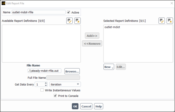
  1. Enter steady-mdot-rfile.out for File Name.
  2. Click OK to close the Edit Report File dialog box.
Save the case file (nozzle_ss.cas.h5).
File → Write → Case...
Initialize the solution.
Solution → Initialization
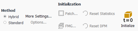
1. Keep the Method at the default of Hybrid.
2. Click Initialize.
Set up gradient adaption for automatic mesh refinement.
You will enable automatic adaption so that the solver periodically refines the mesh in the vicinity of the shocks as the iterations progress. The shocks are identified by their large pressure gradients.
Domain → Adapt → Automatic...
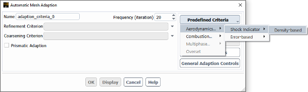
1. Select Aerodynamics... / Shock Indicator / Density-based from the Predefined Criteria drop-down list.
2. Complete the setup in the Automatic Mesh Adaption dialog box.
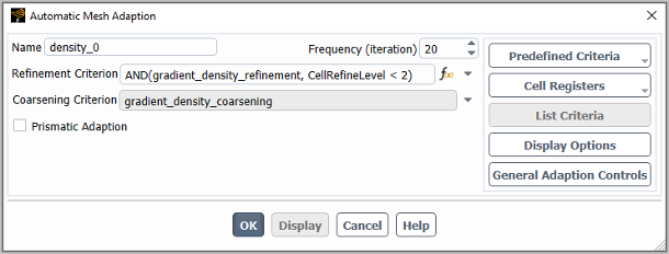
  1. Enter 20 for Frequency (iteration) of mesh adaption.
  2. Click OK to close the Automatic Mesh Adaption dialog box.
Start the calculation by requesting 400 iterations.
Solution → Run Calculation → Run Calculation...
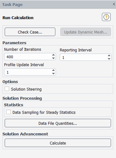
1. Enter 400 for Number of Iterations.
2. Click Calculate to start the steady flow simulation.
Figure 8.3: Mass Flow Rate History
Save the case and data files (nozzle_ss.cas.h5 and nozzle_ss.dat.h5).
File → Write → Case & Data...
Note: When you write the case and data files at the same time, it does not matter whether you specify the file name with a .cas.h5 or .dat.h5 extension, as both will be saved.
Click OK in the Question dialog box to overwrite the existing file.
Check the mass flux balance.
Important: Although the mass flow rate history indicates that the solution is converged, you should also check the mass flux throughout the domain to ensure that mass is being conserved.
Results → Reports → Fluxes...
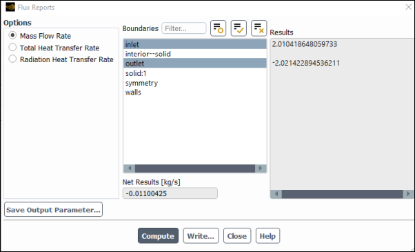
1. Retain the default selection of Mass Flow Rate.
2. Select inlet and outlet in the Boundaries selection list.
3. Click Compute and examine the values displayed in the dialog box.
  
  Important: The net mass imbalance should be a small fraction (for example, 0.1%) of the total flux through the system. The imbalance is displayed in the lower right field under Net Results. If a significant imbalance occurs, you should decrease your residual tolerances by at least an order of magnitude and continue iterating.
4. Close the Flux Reports dialog box.
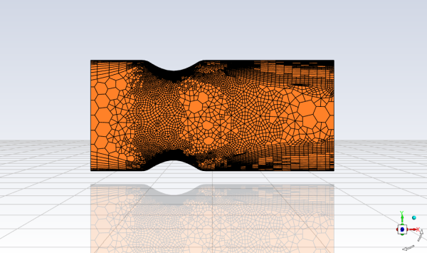
Review a mesh that resulted from the automatic adaption performed during the computation.
Results → Graphics → Mesh → New...
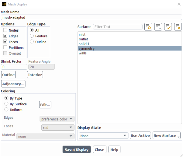
1. Enter mesh-adapted for Mesh Name.
2. Ensure that Edges and Faces are enabled in the Options group box.
3. Select symmetry from the Surfaces list.
4. Click Save/Display and close the Mesh Display dialog box.
  The mesh after adaption is displayed in the graphics window (Figure 8.4: 2D Nozzle Mesh after Adaption).
  Figure 8.4: 2D Nozzle Mesh after Adaption
5. Zoom in by dragging the middle mouse button with the Shift key pressed to view aspects of your mesh.
  Notice that the cells in the regions of high pressure gradients have been refined.
Display the steady flow contours of static pressure.
Results → Graphics → Contours → New...
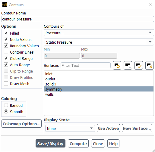
1. Enter contour-pressure for Contour Name.
2. Select Pressure... and Static Pressure from the Contours of list.
3. Select symmetry from the Surfaces list.
4. Click Save/Display and close the Contours dialog box.
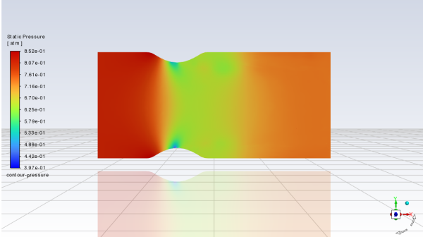
The steady flow prediction shows the expected pressure distribution, with low pressure near the nozzle throat.
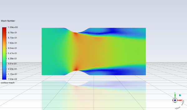
Display the steady-flow contours of mach number.
Results → Graphics → Contours → New...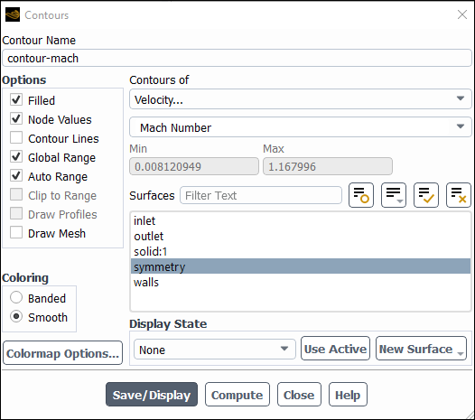
1. Enter contour-mach for Contour Name.
2. Select Velocity... and Mach Number from the Contours of list.
3. Select symmetry from the Surfaces list.
4. Click Save/Display and close the Contours dialog box.

8.4.10. Enabling Time Dependence and Setting Transient Conditions

In this step you will define a transient flow by specifying a transient pressure condition for the nozzle.

Enable a time-dependent flow calculation.
Setup → General
Select Transient in the General task page (Solver group box, under Time).
The pressure at the outlet is defined as a wave-shaped profile, and is described by the following equation:
(8–1)
where
= circular frequency of transient pressure (rad/s)
= mean exit pressure (atm)
In this case, rad/s, and atm.. To convert to SI units multiple by 101325 Pa per atm..
Define the transient boundary conditions at the nozzle exit (outlet).
Setup → Boundary Conditions → Outlet → outlet Edit...
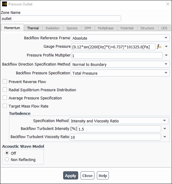
1. Select Expressions from Gauge Pressure drop-down list.
  Enter the following expression for the outlet pressure as a function of time.
  (0.12*sin(2200[Hz]*t)+0.737)*101325.0[Pa]
2. Click Apply and close the Pressure Outlet dialog box.
Update the gradient adaption parameters for the transient case.
Domain → Adapt → Automatic...
1. Select Aerodynamics... / Shock Indicator / Density-based from the Predefined Criteria drop-down list in the Automatic Mesh Adaption dialog box.
2. Enter 25 for Frequency (time-step).
3. Click OK to close the Automatic Mesh Adaption dialog box.

8.4.11. Specifying Solution Parameters for Transient Flow and Solving

Modify the mass_flowrate_out-rfile report file definition.
Solution → Monitors → Report Files → outlet-mdot-rfile Edit...
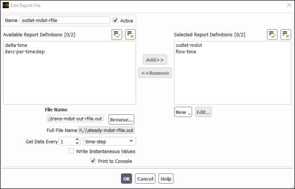
1. Enter trans-mdot-out-rfile.out for File Name.
2. Select time-step from the Get Data Every drop-down list.
3. Click OK to close the Edit Report File dialog box.
Modify the mass_flowrate_out-rplot report plot definition.
Solution → Monitors → Report Plots → outlet-mdot-rplot Edit...
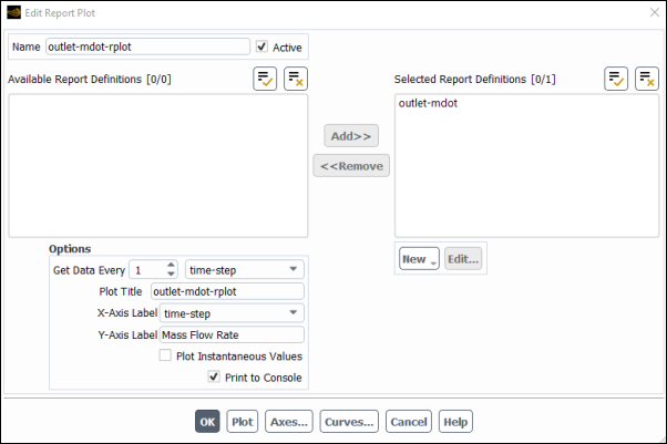
1. For Get Data Every, retain the value of 1 and select time-step from the drop-down list.
2. Select time-step from the X-Axis Label drop-down list.
3. Click OK to close the Edit Report File dialog box.
Save the transient solution case file (nozzle_uns.cas.h5).
File → Write → Case...
Define the time step parameters.
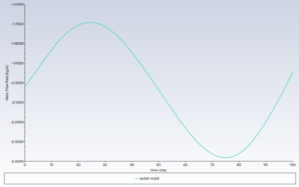
The selection of the time step is critical for accurate time-dependent flow predictions. Using a time step of 2.85596 x 10^-5 seconds, 100 time steps are required for one pressure cycle. The pressure cycle begins and ends with the initial pressure at the nozzle exit.
Solution → Run Calculation → Run Calculation...
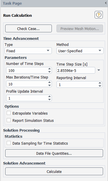
1. Enter 2.85596e-5 s for Time Step Size.
2. Enter 100 for Number of Time Steps.
3. Enter 10 for Max Iterations/Time Step.
4. Click Calculate to start the transient simulation.
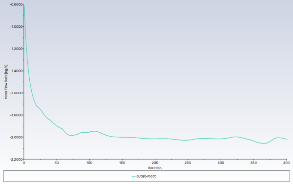
By requesting 100 time steps, you are asking Ansys Fluent to compute one pressure cycle. The mass flow rate history is shown in Figure 8.5: Mass Flow Rate History (Transient Flow).
Figure 8.5: Mass Flow Rate History (Transient Flow)
Optionally, you can review the effect of automatic mesh adaption performed during transient flow computation as you did in steady-state flow case.
Save the transient case and data files (nozzle_uns.cas.h5 and nozzle_uns.dat.h5).
File → Write → Case & Data...

8.5. Summary

In this tutorial, you modeled the transient flow of air through a nozzle. In doing so, you learned how to:

generate a steady-state solution as an initial condition for the transient case.
set solution parameters for implicit time-stepping and apply a user-defined transient pressure profile at the outlet.
use mesh adaption to refine the mesh in areas with high pressure gradients to better capture the shocks.
automatically save solution information as the transient calculation proceeds.

		= circular frequency of transient pressure (rad/s)
		= mean exit pressure (atm)