


To solve a transient problem, you will follow the procedure outlined below:
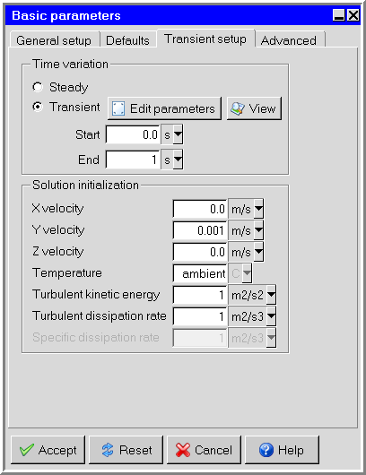
Enable the Transient option in the Transient setup tab of the Basic parameters panel (Figure 26.1: The Basic parameters Panel (Transient setup Tab)). To open the Basic parameters panel, double-click the Basic parameters item under the Problem setup node in the Model manager window.
 Problem setup
 Basic parameters
Enter the starting and ending times for the simulation in the Start and End text fields.
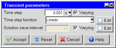
To edit the default transient parameters (if required), click Edit parameters. This will display the Transient parameters panel shown in Figure 26.2: The Transient parameters Panel.
Specify a value for the Time step. The default value is 0.001 s.
Specify whether Ansys Icepak should use a uniform or non-uniform time step.
Enable Varying to specify a non-uniform time step. There are five options in the drop-down list:
Note: If Varying is not enabled, the time step will be uniform.
Linear (ts = i + a t) specifies a linear variation of the time step with time:

(26–1)
where Δt is the time step at time t, Δt0 is the initial time step, and a is a constant. Enter values for the Δt0 and the Factor (a).
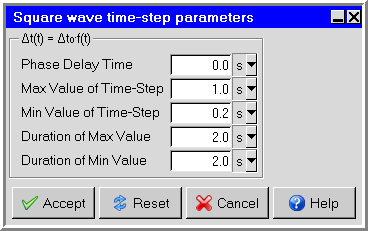
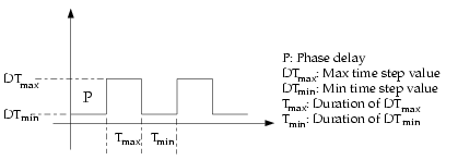
Square Wave specifies a square-wave profile for the time step variation. If the variation of time step required is regular/periodic with time, then this option can be used instead of the Piecewise constant option. To specify a square-wave profile, click Edit to open the Square wave time-step parameters panel (Figure 26.3: The Square Wave Time-Step Parameters Panel).
To understand the meaning of the various parameters in the Square Wave Time-Step Parameters panel, see Figure 26.4: The Square Wave Inputs for Time Step Variation.
Piecewise constant specifies a piecewise constant variation of the time step. Select Piecewise constant in the Transient parameters panel and click Edit. Enter a list of the time/time-step pairs in the Piecewise value pairs (time / time-step) parameters box. It is important to give the numbers in pairs, but the spacing between the numbers is not important. An example of the arrangement of the time/time-step pairs is shown below:

(26–2)
Ansys Icepak will use the time/time-step pairs such that if t< t1 , the time step Δt is given by

(26–3)
Similarly, if t1 ≤t<t 2 ,

(26–4)
Piecewise linear specifies a piecewise linear variation of the time step. Select Piecewise linear in the Transient parameters panel and click Edit. Enter a list of the time/time-step pairs in the Piecewise value pairs (time / time-step) parameters box. It is important to give the numbers in pairs, but the spacing between the numbers is not important. An example of the arrangement of the time/time-step pairs is shown below:

(26–5)
Ansys Icepak will use the time/time-step pairs such that if ts <t≤t1 , the time step Δt is a linear function that varies between Δt0 and Δt1 :

(26–6)
where ts is the Start time specified in the Basic parameters panel, and Δt0 is the Time step increment specified at the top of the Transient parameters panel.
Similarly, for t1 <t≤ t2 , Δt is a linear function that varies between Δt1 and Δt2 :

(26–7)
Automatic time step function is determined based on the estimation of the truncation error associated with the time integration scheme. If the truncation error is smaller than a specified tolerance, the size of the time step is increased; if the truncation error is greater, the time step size is decreased.
An estimation of the truncation error can be obtained by using a predictor-corrector type of algorithm [31] in association with the time integration scheme. At each time step, a predicted solution can be obtained using a computationally inexpensive explicit method (forward Euler for the first-order unsteady formulation, Adams-Bashford for the second-order unsteady formulation). This predicted solution is used as an initial condition for the time step, and the correction is computed using the nonlinear iterations associated with the implicit formulation. The norm of the difference between the predicted and corrected solutions is used as a measure of the truncation error. By comparing the truncation error with the desired level of accuracy (that is, the truncation error tolerance), Ansys Icepak is able to adjust the time step size by increasing it or decreasing it.
In cases where the truncation error remains above the specified tolerance, Ansys Icepak will try to meet the tolerance within 5 attempts. If this tolerance is met, then the iteration moves on to the next time step. An explicit scheme is used to predict the solution at each time step, then the explicit prediction is corrected with an implicit scheme. The truncation error, which is a function of the difference between the predicted and corrected solutions at a specific time is used to calculate the next time step. However, if the calculated truncation error is greater than the tolerance limit, we revert from the currently performed iteration, which is moving from the nth step to n+1th step by performing the iteration with a smaller time step. Since the truncation error is proportional to the time step, decreasing the time step reduces the truncation error. This can be done until the truncation error goes below the tolerance limit.
Specifying Parameters for Automatic Time Stepping
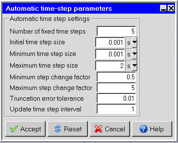
The parameters that control automatic time stepping are in the Automatic time-step parameters panel. This panel is displayed when clicking the Edit button across from Automatic.
Number of fixed time steps specifies the number of fixed-size time steps that should be performed before the size of the time step starts to change. The size of the fixed time step is the value specified for Time step.
It is a good idea to perform a few fixed-size time steps before switching to automatic time stepping. Sometimes spurious discretization errors can be associated with an impulsive start in time. These errors are dissipated during the first few time steps, but they can adversely affect the adaptive time stepping and result in extremely small time steps at the beginning of the calculation.
Important: When the solution tends to exhibit incomplete convergence, rather than increasing the time step size or keeping the same time step size in the next step, Ansys Icepak reduces the time step size by at least half for the next time step (making sure that the time step size does not go below the specified minimum time step size.
Initial time step size specifies the initial time step to be used for the simulation.
Minimum/Maximum time step size specify the upper and lower limits for the size of the time step. If the time step becomes very small, the computational expense may be too high; if the time step becomes very large, the solution accuracy may not be acceptable to you. You can set the limits that are appropriate for your simulation.
Minimum/Maximum step change factor limit the degree to which the time step size can change at each time step. Limiting the change results in a smoother calculation of the time step size, especially when high-frequency noise is present in the solution. If the time step change factor,
 , is computed as the ratio
between the specified truncation error tolerance and the computed
truncation error, the size of time step
, is computed as the ratio
between the specified truncation error tolerance and the computed
truncation error, the size of time step  is computed as follows:
If
 ,
,  is increased to meet the desired tolerance.
If
 ,
,  is increased,
but its maximum possible value is
is increased,
but its maximum possible value is  .
.If
 ,
,  is unchanged.
If
 ,
,  is decreased.
Truncation error tolerance specifies the threshold value to which the computed truncation error is compared. Increasing this value will lead to an increase in the size of the time step and a reduction in the accuracy of the solution. Decreasing it will lead to a reduction in the size of the time step and an increase in the solution accuracy, although the calculation will require more computational time. For most cases, the default value of 0.01 is acceptable.
Update time step interval specifies the number of time steps between the automatic time step adjustment. For example, the default of 1 specifies that a new time step is automatically computed every time step.
Specify the Solution save interval. This value tells Ansys Icepak how often during the solution procedure the results should be saved. Every tenth time step is saved by default.
You can select the Varying button next to the Solution save interval field to set up a piecewise constant interval schedule. Click the Edit button to open the Piecewise constant save interval parameters panel and enter pairs of time save intervals. The save interval value will be dynamically determined for the given flow time from the pairs.
Note:Only steps that have been saved can be used during postprocessing. Large amounts of data can be generated from a transient simulation, so you should decide how much data should be saved for postprocessing. If you are only interested in the solution at the end of the transient simulation, then very little intermediate data need be saved. If you are interested in animating and studying the transient effects in detail, then almost every time step should be saved.
In transient simulations, the .fdat file is saved at regular intervals based on the Solution save interval. The .dat file is saved only at the end of the simulation.
Click Accept in the Transient parameters panel to store the new settings.
Specify the initial conditions for the fluid in your model in the Transient setup tab of the Basic parameters panel (Figure 26.1: The Basic parameters Panel (Transient setup Tab)). For a transient simulation, this corresponds to the initial physical state of the fluid. See Initial Conditions for more details on setting initial conditions.
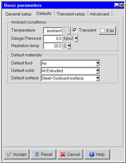
Specify an ambient value of temperature by entering the ambient Temperature under Ambient conditions in the Defaults tab of the Basic parameters panel (Figure 26.6: The Basic parameters Panel (Default tab)).
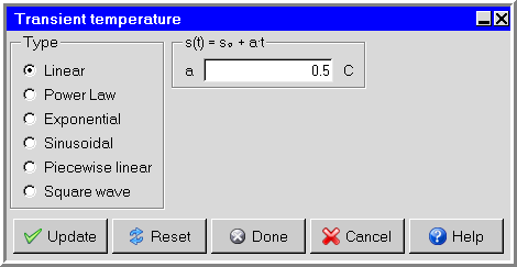
To define the variation of ambient temperature as a function of time, select Transient next to Temperature, and then click Edit. This will open the Transient temperature panel shown in the figures below.
Select the method for the calculation of the variation of ambient temperature with time. The following options are available, and described in more detail in Specifying Variables as a Function of Time.
Linear specifies a linear variation of ambient temperature with time. Enter a value for the coefficient a in Equation 26–9.
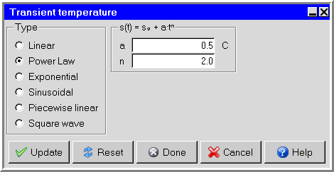
Power law specifies a power law variation of ambient temperature with time. Enter values for the coefficients a and n in Equation 26–10.
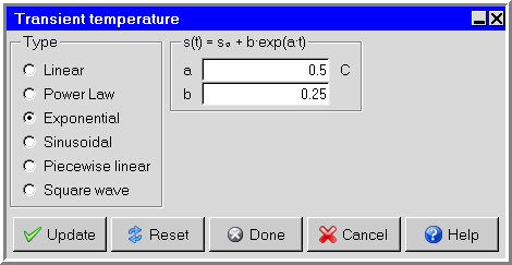
Exponential specifies an exponential variation of ambient temperature with time. Enter a value for the coefficients a and b in Equation 26–11.
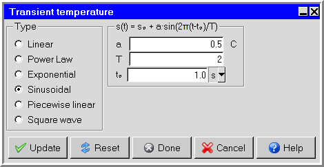
Sinusoidal specifies a sinusoidal variation of ambient temperature with time. Enter values for the period T, the phase shift t0 , and the coefficient a in Equation 26–12.
Piecewise linear specifies a piecewise linear variation of ambient temperature with time. There are two ways to define the piecewise linear variation: the Time/value curve window and the Curve specification panel. These methods are described in Specifying Variables as a Function of Time.
Note: The base temperature specified next to Temperature should be the same value as the ambient temperature at the start of the simulation.
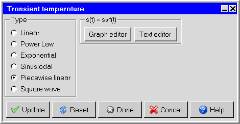
Square wave specifies a square wave variation of ambient temperature with time. Specify the Phase, the On time, the Off time, and the Off value for the square wave, as described in Specifying Variables as a Function of Time.
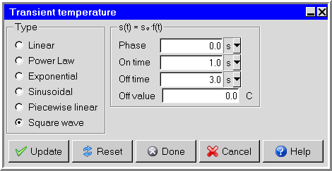
Click Done in the Transient temperature panel when you have finished specifying the variation of ambient temperature with time.
Once you have set the desired parameters in the Basic parameters panel, click Accept to store the new settings.
Specify the transient characteristics of the objects in your Ansys Icepak model. You can specify transient characteristics for the following objects:
Solid or fluid block: Specify the total power as a function of time by selecting the Transient option in the Properties tab of the Blocks panel (see Blocks) and clicking Edit. The Transient power panel used to define the transient power of the block is very similar to the Transient temperature panel. You must also specify the Start time and the End time for the transient simulation for the block.
You can also specify the current as a function of time for Joule heating type inputs by selecting the Joule option in the Properties tab of the Blocks panel (see Blocks) and clicking Edit. From the Joule heating power panel, select the Transient option next to Current and click Edit. The Transient current panel used to define the transient current for Joule heating power of the block is very similar to the Transient temperature panel. You must also specify the Start time and the End time for the transient simulation for the block.
Fan: Specify the transient strength of a characteristic curve fan by turning on Transient strength in the Properties tab of the Fans panel (see Fans) and clicking Edit. The Transient fan strength panel used to define the transient strength of the fan is similar to the Transient temperature panel, except that it contains only the Piecewise linear and Square wave options.
The transient fan strength multiplier scales the total pressure of the fan. The total pressure of the fan is the sum of the static pressure (fan curve) and dynamic pressure:

(26–8)
Opening: For a free opening, you can specify the static pressure, temperature, x velocity, y velocity, or z velocity for flow across the opening as a function of time, by turning on the Transient option in the Properties tab of the Openings panel (see Openings) and clicking Edit. The Transient pressure, Transient temperature, Transient X velocity, Transient Y velocity, and Transient Z velocity panels are very similar to the Transient temperature panel. You must also specify the Start time and the End time for the transient simulation for the opening.
You can also specify the species concentrations as a function of time (see Species Transport Modeling for information on species transport). Select Species in the Openings panel and click the Edit button to open the Species concentration panel. The Transient species panel is used to define the transient species concentrations for the openings.
For a recirculation opening, you can specify the Start time and the End time of the period when the opening is active.
Wall: You can specify the rate of heat transfer through the wall or the temperature on the outer surface of the wall as a function of time, by turning on the Transient option in the Properties tab of the Walls panel (see Openings) and clicking Edit. You can also specify the heat transfer coefficient as a function of time by turning on the Transient option in the Wall external thermal conditions panel. To open the Wall external thermal conditions panel, select Heat transfer coefficient in the Walls panel and click Edit. The Transient power/area, Transient temperature, and Transient heat tr coeff panels are very similar to the Transient temperature panel. You must also specify the Start time and the End time for the transient simulation for the wall.
Conducting thick plate: Specify the total power as a function of time by selecting Transient in the Properties tab of the Plates panel (see Plates) and clicking Edit. The Transient power panel used to define the transient power of the plate is very similar to the Transient temperature panel. You must also specify the Start time and the End time for the transient simulation for the plate.
You can also specify the current as a function of time for Joule heating type inputs by selecting the Joule option in the Properties tab of the Plates panel (see Plates) and clicking Edit. From the Joule heating power panel, select the Transient option next to Current and click Edit. The Transient current panel used to define the transient current for Joule heating power of the plate is very similar to the Transient temperature panel. You must also specify the Start time and the End time for the transient simulation for the plate.
Source: Specify the power as a function of time by turning on the Transient option in the Properties tab of the Sources panel (see Sources) and clicking Edit. The Transient power panel used to define the transient power of the source is very similar to the Transient temperature panel. You must also specify the Start time and the End time for the transient simulation for the source.
For 3D sources, you can also specify the current as a function of time for Joule heating type inputs by selecting the Joule heating option in the Properties tab of the Sources panel (see Sources) and clicking Edit. From the Joule heating power panel, select the Transient option next to Current and click Edit. The Transient current panel used to define the transient current for Joule heating power of the source is very similar to the Transient temperature panel. You must also specify the Start time and the End time for the transient simulation for the source.
Resistance: Specify the total power as a function of time by selecting Transient in the Properties tab of the Resistances panel (see Resistances) and clicking Edit. The Transient power panel used to define the transient power of the resistance is very similar to the Transient temperature panel. You must also specify the Start time and the End time for the transient simulation for the resistance.
Note: The Start time and the End time can be different for different objects.
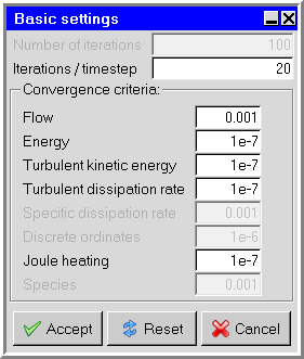
Set the maximum number of iterations to be performed per time step under Iterations/timestep in the Basic settings panel (Figure 26.7: The Basic settings Panel for a Transient Simulation). To open this panel, double-click the Basic settings item under the Solution settings node in the Model manager window. If the Convergence criteria are satisfied before this number of iterations is performed, the solution will advance to the next time step. The default value of 20 iterations/time step should be acceptable for most cases. If you find that the solution is not converging at each time step, you can increase the Iterations/timestep value and/or decrease the size of the Time step increment specified in the Transient parameters panel (Figure 26.2: The Transient parameters Panel).
Start the calculation using the Solve panel. To open this panel, click Run solution in the Solve menu. Click Start solution to start the calculation.
Files will be saved at the frequency specified next to Solution save interval in the Transient parameters panel (Figure 26.2: The Transient parameters Panel). A separate file is saved for each time step for which data are saved.