Using the Power Spectrum for Radiated Field Computations

Suppose we have a single-input linear time-invariant system, and let the input be a random process with power spectral density S_xx(jw). Let the transfer function of the linear system be H(jw). Then we can show that the power spectrum S_yy (jw) of the output is related to that of the input signal as follows:

(46)

If there are N inputs to the system, then it becomes considerably more challenging to compute the power spectrum of the output. In general, the input signals may be correlated to one another. Then the output power spectrum is given by

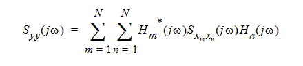
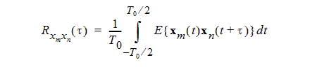
Here x* denotes the complex conjugate of x, and Sx_mx_n (jw) is the cross-power spectral density of the two random signals x_m(t) and x_n(t). This is the Fourier transform of the cross-correlation function Rx_mx_n. For our cyclostationary, real-valued random digital signals the cross-correlation is defined as

Another way of expressing (47) is as a matrix inner product:

(49)

Bipolar Modulation (Statistically Independent Signals)

If the input signals are all uncorrelated then (by definition) Rx_mx_n (t)=0 and Sx_mx_n (jw)=0 for all

mmn. Then the expression for the output power spectrum will simplify to

Equivalently, we could say that the power spectrum matrix in equation (49) becomes diagonal in this case.

The input signals will be uncorrelated if they are statistically independent of one another and we are using bipolar modulation. This is a result of the fact that the expected value of the product of any two bits from different signals is 0.

Unipolar Modulation (Statistically Independent Signals)

If we use unipolar modulation, then the input signals will be correlated, even if the bit patterns for two random digital bit streams are statistically independent of one another. For unipolar modulation, we can show that a cross-correlation between independent bit streams of R^k = 1/4 (for all k) will result. This will produce the cross power spectral density Sx_mx_n(jw).

The derivation of this result is very similar to that for equation (44). Here we have assumed that the two bit streams have the same basic pulse shape. With this result in hand, the power spectrum of the output signal can be computed using equation (47). We can simplify the expression to

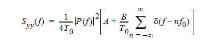
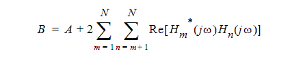
In the above expression

Inputs that Are Not Independent: Differential Signals

Differential signals represent an important special case where two input signals are not at all independent of one another. In the case of bipolar modulation, we can simply write one member of the pair as the negative of the other. The cross-correlation between bits will be -1 for k = 0 and 0 for k m 0. Therefore the cross-power spectral density for the pair will be nonzero. We can show that it will be equal to the negative of equation (41).

Suppose that the two signals of the differential pair are the only inputs to the system and bipolar modulation is used. Then we can use equation (49) to show

For a typical differential pair, the two transfer functions will be nearly equal, and so this expression shows that the output power will be substantially reduced when compared to single-ended signaling.

If we use unipolar modulation for our differential pair, then a bit of value x_m (0 or 1) in one signal becomes 1- x_m (1 or 0, respectively) in the other signal. For two bits in the same period (k =0) the product is always zero, so R_k = 0 for k =0. For two bits in different periods the expected value is ¼ (just as it was for independent unipolar signals), so R_k = 1/ 4 for km0. Plugging this into (48) and simplifying will result in

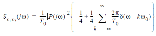
Thus the impulse train part of the cross power spectrum is unchanged (as compared to equation (51) for independent unipolar signals), but now a continuous component has been added. The continuous component of the cross power spectrum is the negative of the continuous component of a self-power spectrum (compare equation (44)).

If we now suppose that the signals of the differential pair are the only inputs to the system, then the output power spectrum has the same form as equation (52), but now the coefficients will be