SBR+ Fast Frequency Looping for High Density Frequency Sweeps

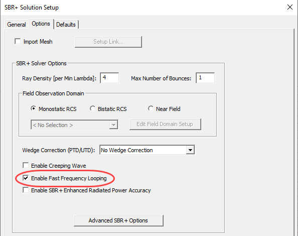
The SBR+ Fast Frequency Looping feature significantly reduces simulation time for high-density frequency sweeps with tens to thousands of uniform frequency samples. The workflow change is simple. In the SBR+ solution type, if you have configured a uniform frequency sweep with at least 2 frequencies, you can switch on the Fast Frequency Looping option in the simulation setup dialog box.

For a standard SBR+ setup:

For a Range Doppler setup:

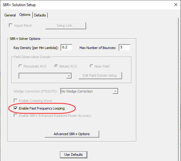
From there, the acceleration is handled automatically, with no other workflow changes in problem setup or post-processing. The acceleration engages for all SBR+ field and signal output types: S-parameters, far-field antenna patterns, near-field E/H-field spatial distributions. Responses from such sweeps are often post-processed outside of Desktop with IFFTs to yield a response as a function of time (or distance) instead of a response vs. Frequency.

Technical Background

An important class of SBR+ applications require high-density, uniform frequency sweeps. These include (inverse) synthetic aperture ((I)SAR) imaging, automotive range-Doppler radar sensing, and 5G coverage fading analysis. More generally, users are interested to Fourier process (IFFT) frequency-domain responses to obtain results in the time domain, which often provides a more intuitive/actionable representation of field and Rx signal behavior. The time-domain representation may be of direct interest, or users may want a corresponding “space-domain” representation by scaling the time axis according to the speed of light. An example of the latter is an mono-static RCS range profile, where the time axis is scaled by half the speed of light (c/2) to correlate scattering features in the response with physical features of the scattering geometry.

Fast Frequency Looping (FFL) significantly reduces simulation time for high-density frequency sweeps where there are tens, hundreds, or even thousands of frequency samples. High sampling density is needed to control aliasing in the time responses. Time (space) resolution improves linearly (Δt and ΔR get smaller) with increasing frequency bandwidth, but if this is not compensated with additional frequency samples to maintain Δf, the uniform interval between frequency samples, aliasing gets correspondingly worse. The aliasing period is inversely proportional to Δf (i.e., smaller Δf and more samples is better).

Like the HFSS FEM and IE solvers, SBR+ is a time-harmonic frequency-domain solver, so frequency samples are added by looping the overall simulation, and run time grows in proportion to the number of frequencies. SBR+ has an important advantage in this regard since the geometric ray paths are frequency independent. For a high-density frequency simulation, the rays are only shot once. Nonetheless, the rays are still processed N_f times in an internal frequency loop. In an SBR+ simulation, one typically observes very little run-time impact in going from 1 to 2 frequencies. However, once N_f reaches 10 or 20 samples, the ray-processing time overtakes geometric ray tracing time, and run time grows linearly with N_f.

TD-SBR+ exploits geometric information in the rays to reduce the computation cost of a high-density frequency sweep to that of simulating at just one frequency. Internally, the long-form SBR+ simulation is performed at just the center frequency. Then, using cached information from each ray path and FFTs, this single-frequency result is efficiently extrapolated to all other frequencies of the uniform sweep. The payoff for hundred-plus frequency samples is typically 5x – 10x.

The workflow change is simple. In the SBR+ solution type, if you have configured a uniform frequency sweep with at least 2 frequencies, you can enable Fast Frequency Looping in the simulation setup dialog box. From there, the acceleration is handled automatically, with no other workflow changes in problem setup or post-processing. The acceleration engages for all SBR+ field and signal output types: S-parameters, far-field antenna patterns, near-field E/H-field spatial distributions.

Because FFL only performs the long-form SBR+ simulation at the center frequency (f_c), it is no longer necessary for excitations to be defined over the entire the entire frequency sweep of the solution setup. For example, imported far-field FFD pattern files only need to be defined at the center frequency, as only that frequency sample will be consulted during the simulation. Likewise, linked sources only need to be simulated at the center frequency in the source design, which can therefore reduce the overall simulation time.

IMPORTANT: When taking advantage of this source simplification while using FFL, it is vital to understand how FFL determines center frequency f_c in order to ensure the source includes the required frequency sample, either as an actual frequency sample in its definition or within the lower and upper extents of the source’s own frequency sweep. The center frequency f_c of the FFL simulation is always one of the frequency samples of the configured uniform frequency sweep, which is not necessarily the average of the lower and upper frequency sample of that sweep. If the number of frequency samples (N_f) is odd, then f_c is the middle sample of the frequency sweep. However, if N_f is even, then f_c is the first sample in the second half the uniform frequency sweep. For example, if the uniform sweep is configured as Linear Count from 9 to 10 GHz and with 100 points, then fc is considered by the FFL simulation to be the 51st frequency sample in that sweep, which is 9.505050505… GHz, not 9.5 GHz. Any source used in that FFL simulation must therefore include 9.505050505 GHz either as an actual frequency sample or within the lower and upper extents of its frequency samples. Otherwise, the simulation will fail with an error message.

In the case of a Range-Doppler setup, the above guidance has a special interpretation. All Range-Doppler setups require a Center Frequency input. SBR+ uses this and other information in the Range-Doppler setup to internally generate a uniform frequency sweep for the simulation. The SBR+ Range-Doppler setup interprets Center Frequency in the exact same manner as FFL. If the number of frequency samples is even, then the user-provided Center Frequency becomes the first frequency in the second half of the uniformly spaced frequency samples. For example, if you configure a Range-Doppler setup with Center Frequency set to 76.5 GHz, and you also switch on Enable Fast Frequency Looping in that setup, then all radar antennas used in that simulation must either have a frequency sample at 76.5 GHz or lower and upper sweep definition that encompasses 76.5 GHz.

Limitations on the Fast Frequency Looping Feature

This feature is:

• Only available in SBR+ Solution Type.
• Limited to uniform frequency sweeps: Linear Step or Linear Count.
  • This includes the ADP Range-Doppler setup option, which is implicitly uniform frequency sampling.
  • Switching on FFL with a non-uniform frequency sweep will result in a validation error.
• Not recommended when relative bandwidth (center frequency divided by absolute bandwidth) exceeds 10 %.
  • The extrapolation is necessarily approximate and only focuses on the impact of changes in the electrical lengths of ray paths and how that causes ray contributions to coherently interfere. This is the typically the dominant source of frequency dependence in response computed by SBR+, but the extrapolation ignores all other sources of frequency dependence:
    • Source antenna pattern or current distribution
    • Distributed sources (arrays and large current-source) with a spread-out time response relative to the time-resolution (bandwidth) of the simulation will not be accurately captured by this acceleration feature, and it is not recommended under those conditions (i.e., if the speed-of-light divided by the absolute bandwidth is smaller than the physical size of the FEBI antenna or the array).
    • Material dispersion: implicit multi-bounce in layered impedance boundaries will only be captured in a composite sense at the center frequency, and multiple internal reflections that would be resolved in the time-domain response at high enough absolute bandwidth will not be resolved when TD-SBR+ is engaged, even if the relative bandwidth remains small.
    • The accelerated FFL results will show increasing deviation from unaccelerated SRB+ results with increasing separation from the center frequency. In many cases, these can appear significant, yet the resulting time-responses after post-processing will remain excellent.
• Simulations that already benefit from GPU acceleration may not show much or any benefit when this feature is engaged. This is because the GPU parallelizes the frequency loop. This feature will engage with or without the GPU processing option, but when run on the GPU, the upshot may be reduced GPU utilization and only slightly faster run time.

• FFL acceleration is well suited to range-Doppler setups. These typically involve hundreds of frequency samples spanning a relative bandwidth that is well under 10%. Under these conditions, FFL will provide 5x – 10x or greater speed-up with little loss of accuracy.”

• FFL requires 4x to 8x more memory for intermediate results when the feature is engaged. If the system does not have enough memory, this can be mitigated by reducing the number of CPU cores while still realizing a net acceleration benefit.

Summary Workflow:

1. Create an HFSS design and set the Solution Type to SBR+
2. Configure the SBR+ design in the usual fashion: sources, excitations, boundaries, materials, near-field and far-field observer domains, etc.
3. In the General tab of the SBR+ Solution Setup dialog
   1. Set the Setup Type to Standard (default) and configure a Linear Count or Linear Step frequency sweep with a large number of frequency samples, OR
   2. Set the Setup Type to Range-Doppler and configure the Range Resolution to be a small fraction of the Range Period (which is typical for such setups). The implied number of frequency samples is Range Period divided by Range Resolution.
4. In the Options tab of the SBR+ Solution Setup dialog box, switch on Enable Fast Frequency Looping
5. Run the simulation
6. Post-process results in usual fashion