
Impedance Boundaries
In HFSS, impedance boundaries represent surfaces of known impedance. The behavior of the field at the surface and the losses generated by the currents flowing on the surface are computed using analytical formulas; HFSS does not actually simulate any fields inside the resistor.
Similar to finite conductivity boundaries, the following condition applies at impedance boundaries:
|  | (1) |
-
 is the is the unit vector that is normal to the
surface.
is the is the unit vector that is normal to the
surface.
- Etan is the component of the E-field that is tangential to the surface.
- Htan is the component of the H-field that is tangential to the surface.
- Zs is the surface impedance of the boundary, Rs + jXs, where
- Rs is the resistance in ohms/square.
- Xs is the reactance in ohms/square.
For example, consider a structure containing two dielectrics separated by a thin-film resistor. This resistor can be represented by an impedance boundary at the surface between the two objects. In the transmission-line equivalent model, the resistor acts as shunt impedance.
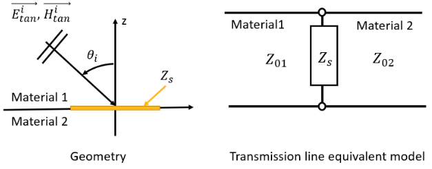
Note that the boundary for that geometry is modified when the Solve Inside flag for an object is set to false. When Solve Inside is false, the boundary is replaced by a half-space material with the surface impedance. This means that the object is treated as perfect magnetic conductor.
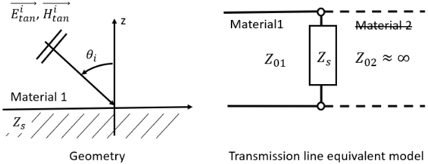
In general, for full-wave solvers, the Solve Inside flag is set automatically based on the material conductivity. The Solve Inside is set to false when the conductivity is greater than Solve Inside Threshold (100000 S/m by default), otherwise it is set to true. Users may override this behavior manually. SBR+ regions do not expose the Solve Inside flag, and such manual override is not available. The only way to modify the behavior of the Solve Inside flag in SBR+ is to modify the global Solve Inside Threshold.