
Emission Test: Set Up and Results
To perform an Emission Test, right-click Results and
select Create Report. For Report Type, select Emission Test (Fig. 4).
It is not necessary to define a Radiation Near Field Setup in advance
- the software will do this automatically for you.
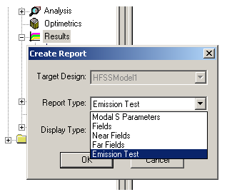
Fig. 4 Preparing an Emission Test
The simplest form of the Emission Test does not take
the actual spectrum of your digital signal into account. This is the
case for the first four spheres under Quantity (Fig. 5). For every frequency,
the source excitation is the same power or voltage (depending on your
model and your settings under Fields/Edit Sources), and the maximum |E|
on the sphere is reported (Fig. 6).
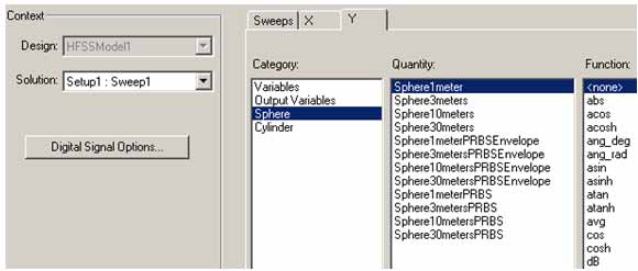
Fig. 5 Selecting an
Emission Test at one meter distance from the origin,
without scaling for the spectrum of the actual signal
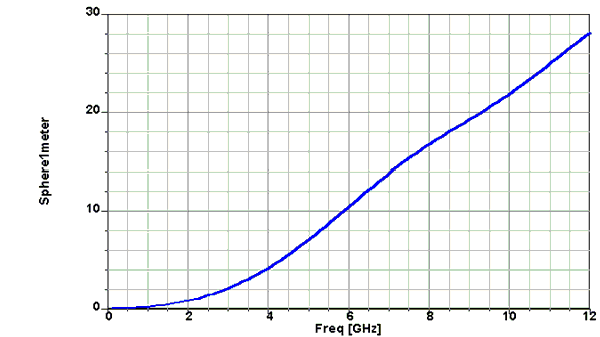
Fig. 6 Result of the Emission Test of Fig. 5
In principle, the data in Fig. 6 can be compared with EMC regulations. However, in practical situations one wants to scale these data by taking the spectrum of the actual digital signal into account. To do this, specify your rise time and hold time under Digital Signal Options (Fig. 5) and select one of the spheres with PRBS in the name under Quantity (Fig. 5). PBRS stands for Pseudo-Random Binary Sequence.
In this example, we look at a digital signal with a rise
time of 200 ps and a hold time of 800 ps (Fig. 7). We plot the maximum
|E| on a one-meter sphere around the origin with two weighting functions:
the exact one, which has many zeroes, and "envelope", which shows the
envelope. Figure 8 shows the result.
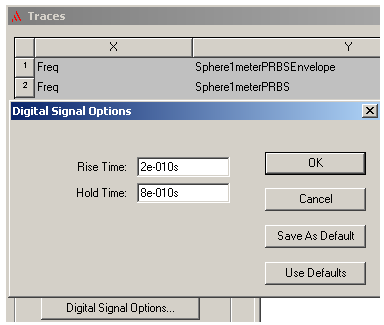
Fig. 7 Setting up an Emission Test with scaling for the spectrum of the digital signal
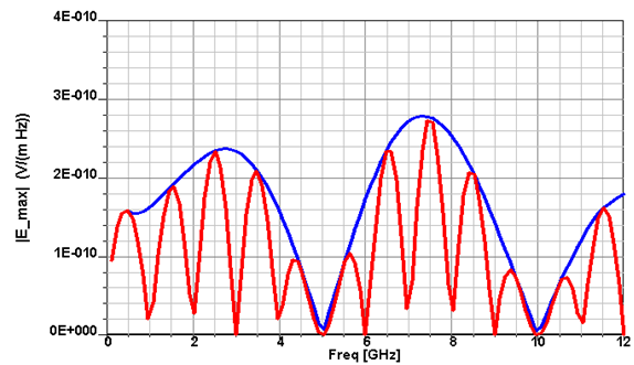
Fig. 8 Emission Test
for a pseudo-random digital signal.
Red: exact scaling; blue: envelope scaling.
Scaling factor
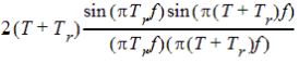
The red line in figure 8 is the result of multiplying figure 6 by
|  | (1) |
where T is the hold time, Tr is the rise time, and f is the frequency. If figure 6 corresponds to a situation where the source produces an AC signal with an amplitude V0 (peak-to-peak swing 2V0) at every frequency, then figure 8 corresponds to a situation where the source produces a PRBS with levels ±V0 (a swing of 2V0) and the given hold and rise times. Let's make a sanity check at 7.5 GHz. For our digital signal, at this frequency, the factor becomes
| (2) | |
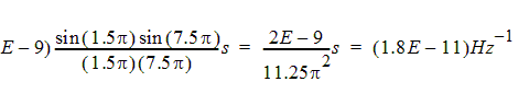
Indeed, |Emax| in Fig. 6 is 16 V/m at 7.5 GHz, and in Fig. 8 the value is 280 pV/(m Hz).
Comparison with regulations
How does this level relate to EMC regulations? First of all, one has to take into account that EMC regulations specify a bandwidth of the measurement equipment of at least 100 kHz. The level of 2.8E-10 V/(m Hz) would register 28 µV/m when measured with equipment of which the bandwidth is 100 kHz (or a little over 100 kHz with roll-off at the edges). Typical MIL-STD EMC limits are on the order of several hundred µV/m at 1m. Hence, this simple, admittedly unrealistic example stays well within the limits. One reason is that its considerable power is spread out over a very broad range of frequencies. A regular clock pulse transmitted by this device would have its power concentrated in narrow bands and would certainly violate regulations. Another reason why the spectral density is low is that 7.5 GHz is well beyond the knee frequency of 0.35/Tr = 1.8 GHz.
Why is the envelope function provided?
Note that the red line in Fig. 8 has many zeroes in the frequency spectrum. There are two reasons for providing the envelope function.
- If you would produce a frequency sweep and/or a plot with a small number of points, many points would be likely to lie in the valleys and you might not distinguish the peaks anymore. This would give you a false impression.
- The red line is based on the assumption of bits with perfect trapezoidal shapes. In reality, your signal would not have been perfectly trapezoidal when it was generated, and may have suffered some additional distortions due to interactions in your device. This reduces the value of the fine structure in the spectrum.
Result for a regular clock pulse
The spectrum of a repetitive clock signal is very different from the spectrum of a pseudo- random binary sequence: it consists of narrow spikes. The Emission Test in Fig. 6 can be used to produce the radiated spectrum of a clock pulse. For example, if we have a clock pulse with zero rise time and fc=1GHz, we would take the points at 1 GHz, 3 GHz, 5 GHz, 7 GHz, etc., and multiply those fields by 2/p, 2/(3p), 2/(5p), 2/(7p), etc. It would look like the following figure.
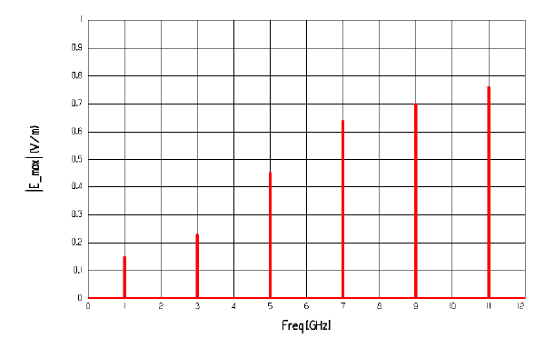
Fig. 9 Emission Test for a clock pulse with a clock frequency of 1 GHz
Whereas the PBRS satisfied strict military standards, the clock pulse violates them by several orders of magnitude. This is because the spectrum of a clock pulse is concentrated in narrow high spikes.