Conclusions and Discussion
This note has dealt with the output responses of linear systems with deterministic (finite energy as well as periodic) and stochastic (random) inputs.
When the signals are deterministic, and have the same time-domain waveforms (apart from constant scaling factors) it is fairly straightforward to consider multiple inputs and compute the Fourier transform of the output signal. The Fourier transform could be a continuous function of frequency (for finite energy signals) or a set of sharp lines (for periodic signals.)
If the signals are random, the process of combining multiple inputs is more complex. In addition to the power spectrum for each input, we must also know the cross power spectrum for every pair of inputs. The cross power spectrum depends on whether the inputs are statistically independent or not. We saw that differential signals are an important special case where signals are strongly dependent on one another. Despite all of these complications, it is still possible to compute the output signal power, and the procedure is sufficiently mechanical for it to be reduced to a computer program.
In this note we have focused our attention on random binary-valued logic signals. These are the sorts of signals we expect to see on the internal buses of a digital system. There are other random signal types (not considered here) that could be of interest. One class that is worthy of mention is digital communication signals, such as PAM, CPM, CPFSK, QPSK, etc.
Appendix A: Handy Delta Function Facts
Definition of the Dirac Delta Function
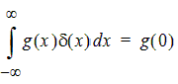
The Dirac delta function d(x) is defined by the following relations:


Delayed Delta Functions
Using Property 3 above, and a change of variables, we can show that if the delta function is shifted:

Time Reversal of a Delta Function

Thus a time reversal has no effect on the basic properties of the delta function.
Products of Delta Functions with Regular Functions
It is easy to see that
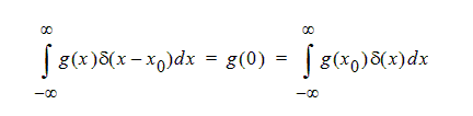
Thus we are free to replace g (x)d( x-x0) by g( x0) d(x -x0), or vice versa.
Scaling the Argument for Delta Functions
This often occurs when converting from angular frequency (radians/s) to Hertz. Let A be a positive, constant scale factor and define u =Ax. Then we can show

Therefore, we can replace

When A =2p, we have the common case of converting from w to f.
The above discussion can also be used to explain the units associated with a delta function. The definition of the delta function requires that its argument should be dimensionless. Nonetheless we often write expression like d (t- t0) where the argument is a variable (for example, time) with physical dimensions (seconds in this case.) To reconcile this with the definition, we must introduce a scaling factor. Suppose we introduce a dimensionless time variable t such that t =(1s)t. Then the scaling factor A = 1s (1 second) and we have

Thus a delta function implicitly carries units of 1/[units of its argument.]
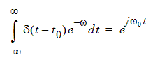
Fourier Transform of a Delta Function in Time
Using the definition of the Fourier transform and the definition of the delta function, we get
Inverse Fourier Transform of a Delta Function in Frequency
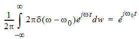
Using the definition of the inverse Fourier transform, we have
Fourier Transform of an Infinite Train of Impulses
Suppose we have an infinitely long "train" of time-domain impulses:
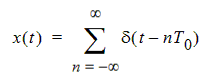
This is a periodic signal. Its Fourier coefficients are

Therefore we can represent the signal as its Fourier series

The Fourier transform is then easily found from one of the above relationships:
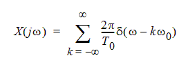
where w0 = 2p /T0. If we prefer to measure frequency in units of Hz, this becomes
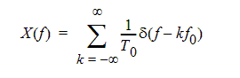
where f0 = 1/T0. Thus we have shown that the Fourier transform of an infinite impulse train is another infinite impulse train.
The same thing works for a frequency-domain train of impulses. We have

The Fourier series coefficients are

Thus

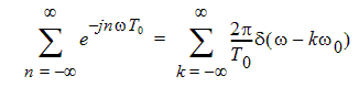
This can be used to prove the useful fact that