


You can specify loads with simple tables of numeric data. Enter data by using the Magnitude property of the boundary condition or equivalent property. (For example, you can enter tabular data for Displacements by using the Distance property.)
Tabular Data vs. Tables
Mechanical supports two ways to specify a load with tables of numeric data:
Tabular data (described in this section) represents simple tables of magnitude that are entered directly into Mechanical. For example, for Force, you can enter a table of the magnitude of the force on the boundary versus time.
Tables allow you to create more complex tabular loads with multiple independent and dependent variables. You can import tables from external data files or directly enter them into Mechanical. For a list of analysis systems that support tables and instructions on how to assign them to boundary conditions, see Specifying Loads With Tables.
Entering Tabular Data
In the Details pane, click Magnitude (or the equivalent field name) and select from the fly-out menu.

Alternatively, you can add tabular data by specifying a Constant value for the Magnitude and entering additional values in the Tabular Data window. For details, see Converting Constant Magnitudes to Tabular Magnitudes.
Enter the tabular data in the Tabular Data window (pressure, force, frequency, and so forth). Enter new values into the row that begins with an asterisk (*), regardless of whether the time or frequency point is higher or lower than the last defined point in the table. The application automatically sorts the content of the table into ascending order. Tabular Data allows up to 100,000 entries.
Viewing and Plotting Tabular Data
The Graph window displays the variation of a tabular load with time for Static and Transient analysis systems or frequency for Harmonic analysis systems.
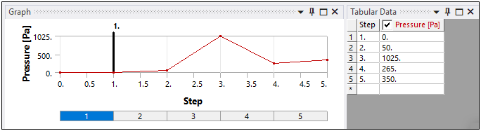
The components of the load are color-coded to match the column name in the Tabular Data window. A check mark in the column title specifies whether that component is plotted in the Graph window. To turn off the plot, clear the check box.
Tabular Data values that are preceded by an equal sign (=) are not defined table values. These values are interpolated by the application and are shown in the table for reference only.
Clicking on a time value in the Tabular Data window or selecting a row in the Graph window will update the display in the upper left corner of the Geometry window with the appropriate time value and load data.
For time varying loads, annotations in the Geometry window display the current time in the Graph window along with the load value at that time.
For frequency varying loads, annotations in the Geometry window displays the minimum range of harmonic frequency sweep and load value of first frequency entry.
Activating and Deactivating Load Steps
You can activate or deactivate individual steps in a tabular load. If you wish for a load to be active in some steps and removed in other steps, follow the directions in Activating and Deactivating Loads.
Spatial Load Tabular Data
When using spatial varying loads, selecting Tabular as the input option displays the Tabular Data category and based on the entry of the Tabular Data category, the Graph Controls category may also display.
The Tabular Data category provides the following options:
- Independent Variable
The Independent Variable property specifies how the load varies with either (default), load (Static Structural only), or in the , , or spatial direction. For a Harmonic Response analysis, the default setting is Frequency, unless you set the Non-Cyclic Loading Type property to either or , in which case, for the supported loading types, the default setting is or . And, for certain temperature-based loads, you can select as the Independent Variable.
Note:The application typically writes loading values to the input file as a table of values. When you set the Independent Variable property to , the application instead writes a constant load value for each load step.
For a Pressure load, the Define By property must be set to .
The option becomes available for Line Pressure loads in a 3D analysis when the Define By property is set to or Pressure loads in a 2D analysis when the Define By property is set to .
The option enables you to define pressure as a function of the distance along a path whose length is denoted by . When you select the variable, the Tabular Data window accepts input data in the form of normalized values of path length () and corresponding Pressure values. A path length of 0 denotes the start of the path and a 1 denotes the end of the path. Any intermediate values between 0 and 1 are acceptable in the table. Load values are sent to the solver for each element on the defined path based on a first-order approximation.
- Coordinate System
The Coordinate System property displays if you specify the Independent Variable in a spatial direction (X, Y, or Z). Use this property to specify a coordinate system.
- Graph Controls
The Graph Controls category displays when you define the Independent Variable as a spatial direction (X, Y, or Z), as , or as . This category provides the property X-Axis which you use to change the Graph window's display. The options of the X-Axis property vary based upon analysis type and the selection made for the Independent Variable property. Options may include , or the spatial direction specified, or .
When the X-Axis property is defined as Time:
Tabular Data content can be Scaled against time.
You can Activate and/or Deactivate the load at a solution load step.
If is not an available option of the X-Axis option, then scaling or activation/deactivation are not possible for the boundary condition.