


The generic details of how to read CGNS files and the file structure are fully documented in the documentation available from the CGNS website.
In the following sections, it may be useful to work from an example of the CFX preprocessing setup in this case. The following flow solver CCL was created using a transient version of the CFX axial turbine MFR tutorial:
 OUTPUT CONTROL:
     EXPORT RESULTS: export1
       Option = Surface Data
       EXPORT FORMAT:
         Filename Prefix = trouser
         Option = CGNS
       END
       EXPORT FREQUENCY:
         Option = Time Interval
         Time Interval = 2.124E-5 [s]
       END
       EXPORT SURFACE: rotatingdipole
         Option = Acoustic Rotating Dipole
         Output Boundary List = Blade
       END
       EXPORT SURFACE: regulardipole
         Option = Acoustic Dipole
         Output Boundary List = Shroud,Shroud 2
       END
     END
     EXPORT RESULTS: export2
       Option = Surface Data
       EXPORT FREQUENCY:
         Option = Time Interval
         Time Interval = 2.124E-5 [s]
       END
       EXPORT SURFACE: dipole
         Option = Acoustic Dipole
         Output Boundary List = Blade 2
       END
     END
  END
In this example, the user has selected to output two different groups of files
corresponding to the two objects, export1 and
export2, at the same time interval. The object names could
be any string and by default the object name is used as the file prefix unless the
user overrides that by setting the Filename Prefix option under
EXPORT FORMAT.
For export1, the user has selected to output a rotating dipole surface source
called rotatingdipole on the boundary called
Blade (which happens to be in a rotating domain). In
addition, a regular dipole source, called regulardipole, will
be written on boundaries Shroud and Shroud
2. In this example, Shroud is in a rotating
domain and Shroud 2 is in a stationary domain. This is an
example of where the flow solver will split the surface source into two different
regions because the surface spans across two CFX domains.
For export2, they have selected to output a dipole source,
called dipole, on Blade 2, which is in a
stationary domain.
The export surface names in both cases are also provided by the user, in addition to the export results names, during CFX pre-processing.
The tree structure of the export2 results output looks as
follows:
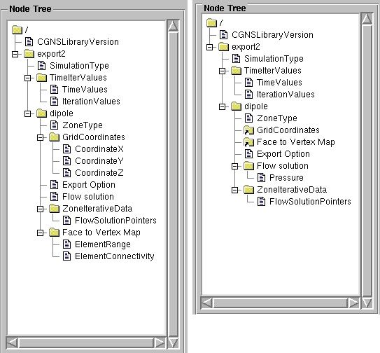
On the left is the grid file and on the right is a solution file. All CGNS files
contain a root node called "/" and are set up like a file system
below that root node. Below the root node is CGNSLibraryVersion, which gives the
CGNS version used to write the file. Both mesh and solution files contain a base
node called export2, which corresponds to the results object
name and the file prefix. Below that node, the following nodes are defined:
SimulationType simply contains a string stating that the
solution is written from a time-accurate or nontime-accurate simulation.
Acoustic output will always be from a time-accurate simulation in CFX.
TimeIterValues is a
BaseIterativeData_t node that contains the time
values and timestep data for the solutions in the file.
TimeIterValues/TimeValues is a
DataArray_t node that contains a list of real
values corresponding to the simulation times stored in the file. In our case,
there is only ever one time value inside a single CGNS file.
TimeIterValues/IterationValues is also a
DataArray_t node that contains the integer value
corresponding to the timestep number. This number is exactly the same as that
encoded in the file name.
dipole is a CGNS Zone_t node
and contains the grid coordinates and nodal area vectors in the mesh file. The
solution file contains the boundary pressures and links back to the grid
coordinates and the element to vertex map.
ZoneType is a processor_t
node that contains the type of grid written to the file and is always set to
Unstructured. This is a default CGNS name.
Export Option is written for all regions and contains a
string that tells what kind of surface export option was used to create the
data. In the two examples, this string will be either Acoustic
Dipole or Acoustic Rotating Dipole.
Flow Solution is a
FlowSolution_t node that contains the solution
values below it written on the element nodes. In the mesh file, this directory
contains nothing for this case because the file only contains data for a dipole
source. For rotating dipole source cases, this directory contains the nodal area
vector components called Nodal Area VectorX,
Nodal Area VectorY, Nodal Area
VectorZ. (Normally, the CGNS documentation has a suggested naming
convention for variables written to FlowSolution_t
nodes. There is no suggested name for Nodal Area Vectors
but this format follows the suggested naming convention for vectors.)
ZoneIterativeData is a
ZoneIterativeData_t node that contains a single
node below it called FlowSolutionPointers. This node is a
DataArray_t node that contains an array of
character strings pointing to the directory names for flow solutions at
different timestep values. Because only one timestep is written to each CGNS
file, this node only holds one character string called Flow
Solution.
GridCoordinates is a
GridCoordinates_t node that contains the surface
mesh <x,y,z> coordinates in the flow solver coordinate system.
CoordinateX/Y/Z are just
DataArray_t nodes with the grid coordinate
components.
Face to Vertex Map is an
Elements_t directory node that contains the
element range and connectivity.
Face to Vertex Map/ElementRange is an
IndexRange_t node that gives the range of
elements assigned to the region. In all cases, this node gives two numbers 1 and
N, where N is the number of surface elements written for the region.
Face to Vertex Map / ElementConnectivity is a
DataArray_t node that contains the fact to
vertex map for each boundary face (2D QUAD_4)
element. An example of this array with both triangular and quadrilateral faces
is as follows:
465 152 155 155
459 176 178 178
579 154 157 157
579 156 154 154
465 157 152 152
2 32 31 1
1 31 462 461
3 33 32 2
4 34 33 3
5 35 34 4
6 36 35 5
7 37 36 6
8 38 37 7
9 39 38 8
The first five elements on this boundary are actually triangular faces written
as degenerate quadrilaterals. The remaining elements are real quadrilaterals.
The elements are always written to the file with the CGNS element type
QUAD_4.
GridCoordinates is only a link node that gives the
filename of the mesh file corresponding to the solution.
Face to Vertex Map is another link node that gives the
filename of the mesh file corresponding to the solution.
FlowSolution/Pressure is a
DataArray_t node that contains the boundary
pressures on element vertices.
The last example shows a case where the dipole export surface has been broken into two regions because the boundary list spans across more than one CFX domain. In this case, one domain is rotating (R1) and the other is stationary (S2):
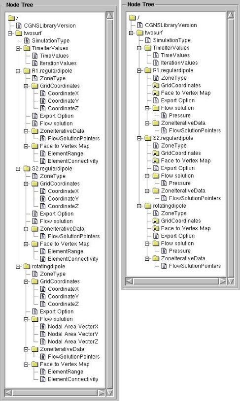
The main difference between this example and the last one is that the split regions have been prefixed with the corresponding CFX domain name and a period character. All other nodes contain the exact data as the simple case previously described.