


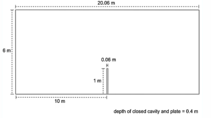
This tutorial uses an example of an oscillating plate within a fluid-filled cavity. A thin plate is anchored to the bottom of a closed cavity filled with fluid (air), as shown in the image below.
A thin plate is anchored to the bottom of a closed cavity filled with fluid (air), shown below. There is no friction between the plate and the side of the cavity. An initial pressure of 100 Pa is applied to one side of the thin plate for 0.5 s to distort it. Once this pressure is released, the plate oscillates back and forth to regain its equilibrium, and the surrounding air damps this oscillation. You will simulate the plate and surrounding air for a few oscillations to be able to observe the motion of the plate as it is damped.
The case is set up as a two-way FSI co-simulation. It models the motion of the oscillating plate using a Mechanical Transient Structural analysis and the motion of the fluid in the closed cavity using a Fluid Flow (CFX) analysis. The two analyses are coupled and then solved at the same time (co-simulation), with Maxwell coordinating the solution process and the data transfers between the two participants.
- Data Transfers
The two-way coupling involves two data transfers:
Force: Force data from the motion of the air are received by the transient structural analysis, which models the structural behavior over time.
Displacement: Displacement data from the motion of the plate are received by the fluid-flow analysis as it solves the fluid behavior over time.
- Transient Settings
The oscillation of the plate is dependent on time, so appropriate time values have been specified for the coupled transient analysis:
End Time: This is the total time observed for the analysis. The time duration is set to 10 s, which is enough time to observe the oscillating plate a few times.
With this time duration, the analysis does not model the full damping back to the plate's equilibrium. When setting up a transient analysis, make sure that you choose a time duration that will allow you to observe the behavior of interest in the system.
Time Step Size is the length of the time increments that you are solving within the transient analysis. The time step is set to 0.1 s, which is fine enough to observe the oscillations to a reasonable degree.
When setting up a transient analysis, make sure you choose a time step that works for the physics you are solving. Too large a time step will miss behavior of the system, and too small a time step will be computationally expensive.