To use the aero-optics model to calculate the aero-optical distortion, perform the following steps:
Read in a mesh. You must ensure that there are separate boundary zones of type wall to represent the optical aperture for each optical beam that you want to define. These boundary zones should be sufficiently resolved for your beam grid, as the ray lines will originate from the face centroids. The entire domain should be larger than your area of interest.
Set up your fluid flow problem, so as to resolve all of the optically relevant spatial and time scales. Note that the aero-optical distortion and the unsteady density field will have more accurate results if you use the density-based solver.
Open the Aero-Optics dialog box.
 Setup → Models →
Aero-Optics
Setup → Models →
Aero-Optics  Edit...
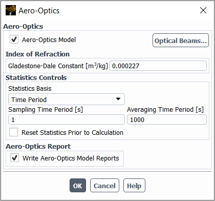
 Enable the Aero-Optics Model option.
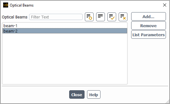
Click the button to open the Optical Beams dialog box, where you can manage the optical beams that are evaluated during the calculation.
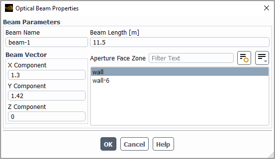
Click the button to open the Optical Beam Properties dialog box, where you can define an optical beam.
Enter a Beam Name for this definition.
Make a selection from the Aperture Face Zone list to specify the zone that represents the optical aperture. Each of the face zones available here are of type wall.
Note: You must use a unique face zone for each beam.
Enter a value for the Beam Length. It is recommended that this length be sufficient to extend past the near-wall region, through all of the turbulent and flow structures of interest. This corresponds to
 in Equation 11–3.
Enter values for the X Component, Y Component, and (for 3D cases) Z Component to define the Beam Vector. You will likely want to direct the beam through any highly turbulent regions, shocks, or other inhomogeneous flow field features in order to evaluate the optical distortion.
Click to close the Optical Beam Properties dialog box.
You can repeat the previous step if you would like additional optical beam definitions.
After you have created one or more definitions, you can use the Optical Beams dialog box to take additional actions prior to running the calculation. If you make a selection from the Optical Beams list, you can use the buttons at the right of the dialog box:
Click to delete the selected definition.
Click to print the attributes of the current selection in the console.
Click in the Optical Beams dialog box when you are done managing the optical beams.
In the Aero-Optics dialog box, enter a value for the Gladstone-Dale Constant (
 in Equation 11–2)
that is used to determine the Index of Refraction for your fluid
medium.
in Equation 11–2)
that is used to determine the Index of Refraction for your fluid
medium.For steady calculations, enter the Sampling Iterations (that is, the iterations per sample) in the Sampling Controls group box.
For transient calculations, define how the fluid density field is sampled in the Statistics Controls group box:
You can select Time Period from the Statistics Basis drop-down list, and then define the Sampling Time Period and Averaging Time Period in seconds, that is, the time period for the sample and the averaging window, respectively.
You can select Time Steps from the Statistics Basis drop-down list, and then define the Sampling Time Steps and Averaging Time Steps, that is, the number of time steps per sample and averaging window, respectively.
When determining the settings for sampling the flow data for the aero-optics model calculations, note that it is proved by Wang et al. [7] that an adequately resolved LES can capture all relevant optical time and spatial scales. Therefore you have the freedom to choose a high sampling frequency at every fluid time step or to decrease it to a sample at every 10 time steps or more, based on the turbulence characteristic of the given case.
(Optional) For transient calculations, you can enable the Reset Statistics Prior to Calculation option if you want the running average of the collected density field for the aero-optical sampling to be reset before the next calculation. Note that you can return to this dialog box and change this option at any point between calculation runs, depending on when you want to reset the statistics.
(Optional) Enable the Write Aero-Optics Model Reports option if you want a data file to be saved in the working directory during transient calculations for each optical beam. Note that these files contain quantities (as listed below) that are not otherwise available through postprocessing in Fluent. The files are named
optics-report-case_<case_name>-start-time_<start_time>-beam-name_<beam_name>.csv. These files can be viewed in a text editor after the calculation to evaluate the following quantities at every time step:Piston
This represents
 in Equation 11–9 and Equation 11–10.
Tip
This represents
 in Equation 11–9 and Equation 11–10.
Tilt
This represents
 in Equation 11–9 and Equation 11–10.
The root mean square of the optical path difference
The time-averaged value of the root mean square of the optical path difference
Click in the Aero-Optics dialog box to save the settings.
(Optional) You can control the level of detail about the aero-optics model that is printed in the console during the calculation by using the following text command:
define→models→optics→verbosityRun the calculation.
Postprocess your results. The following field variables are available under the Optics... category, and they can be evaluated on the face zones on which the optical beams were defined:
Optical Path Length (for steady and transient calculations)
This represents
 in Equation 11–4.
Optical Path Length (Time-Averaged) (for transient calculations only)
This represents
 in Equation 11–4, the
time-averaged value of the optical path length, accumulated for the current averaging window.
Note that this field variable might still be evolving, depending on where in the averaging
window the calculation stopped; to ensure that you have a mature value (that accounts for a
full averaging window), you can instead use the Optical Path Length (Time-Averaged,
Previous).
in Equation 11–4, the
time-averaged value of the optical path length, accumulated for the current averaging window.
Note that this field variable might still be evolving, depending on where in the averaging
window the calculation stopped; to ensure that you have a mature value (that accounts for a
full averaging window), you can instead use the Optical Path Length (Time-Averaged,
Previous).Optical Path Length (Time-Averaged, Previous) (for transient calculations only)
This represents
 in Equation 11–4, the
time-averaged value of the optical path length, accumulated for the previous averaging window
(so it is guaranteed to be mature, that is, no longer evolving due to averaging).
in Equation 11–4, the
time-averaged value of the optical path length, accumulated for the previous averaging window
(so it is guaranteed to be mature, that is, no longer evolving due to averaging).Optical Path Length (Fluctuations) (for transient calculations only)
This represents
 in Equation 11–4.
Optical Path Difference (Total) (for steady and transient calculations)
This represents
 in Equation 11–5.
Optical Path Difference (Steady-Lensing Component) (for transient calculations only)
This represents
 in Equation 11–5 and Equation 11–6, accumulated for the current averaging
window. Note that this field variable might still be evolving, depending on where in the
averaging window the calculation stopped; to ensure that you have a mature value (that
accounts for a full averaging window), you can instead use the Optical Path
Difference (Steady-Lensing Component, Previous).
in Equation 11–5 and Equation 11–6, accumulated for the current averaging
window. Note that this field variable might still be evolving, depending on where in the
averaging window the calculation stopped; to ensure that you have a mature value (that
accounts for a full averaging window), you can instead use the Optical Path
Difference (Steady-Lensing Component, Previous).Optical Path Difference (Steady-Lensing Component, Previous) (for transient calculations only)
This represents
 in Equation 11–5 and Equation 11–6, accumulated for the previous averaging
window (so it is guaranteed to be mature, that is, no longer evolving due to
averaging).
in Equation 11–5 and Equation 11–6, accumulated for the previous averaging
window (so it is guaranteed to be mature, that is, no longer evolving due to
averaging).Optical Path Difference (Steady-Lensing Component Removed) (for transient calculations only)
This represents
 in Equation 11–5.
Optical Path Difference (Low-Order Component) (for transient calculations only)
This represents
 in Equation 11–8 and
Equation 11–9.
in Equation 11–8 and
Equation 11–9.Optical Path Difference (High-Order Component) (for transient calculations only)
This represents
 in Equation 11–8.
Important: When viewing contours of the field variables in the Optics... category, you must disable the Node Values option in order to establish the minimum and maximum for the range of values. After the range is calculated, you can enable the Node Values option as needed.