32.11. Example

The following example demonstrates an end-to-end workflow in Fluent where you import a CAD geometry into the Watertight Geometry Meshing workflow, proceed through various meshing tasks to generate a volume mesh, switch to the solver where you will setup, solve, and postprocess a CFD analysis:

Prepare to run this example with a simple CAD geometry:
1. Download the exhaust_manifold.zip file here .
2. Unzip exhaust_manifold.zip to your working directory.
  The SpaceClaim CAD file manifold.scdoc can be found in the folder. In addition, the manifold.pmdb file is available for use on the Linux platform.

Create a computational mesh.

Start Fluent in Meshing Mode.
In the Fluent Launcher, select the Meshing workspace, enable Show Beta Launcher Options, and enable the Python Console (Beta) option under General Options and click Start.
Once Fluent is opened, you can start working in the Python Console.

Initialize the Watertight Geometry meshing workflow, and set the default global units for length, area, and volume:

>>> workflow.InitializeWorkflow(WorkflowType=r'Watertight Geometry')
>>> meshing.GlobalSettings.LengthUnit.set_state(r'mm')
>>> meshing.GlobalSettings.AreaUnit.set_state(r'mm^2')
>>> meshing.GlobalSettings.VolumeUnit.set_state(r'mm^3')

Import the CAD geometry.

First, a CAD geometry file's name and location are specified, and task updated:

>>> workflow.TaskObject['Import Geometry'].Arguments.set_state({r'FileName': r'C:/sample/manifold.scdoc',})
workflow.TaskObject['Import Geometry'].Execute()

Add local sizing.

Keep the default settings and update the task:

>>> workflow.TaskObject['Add Local Sizing'].AddChildAndUpdate()

Generate the surface mesh.
Keep the default settings and update the task:
```
>>> workflow.TaskObject['Generate the Surface Mesh'].Execute()
```

Describe the geometry.

In this task, the workflow needs a description of the CAD geometry.

>>> workflow.TaskObject['Describe Geometry'].UpdateChildTasks(SetupTypeChanged=False)
>>> workflow.TaskObject['Describe Geometry'].Arguments.set_state({r'CappingRequired': r'No',
r'SetupType': r'The geometry consists of only solid regions',})
>>> workflow.TaskObject['Describe Geometry'].UpdateChildTasks(SetupTypeChanged=True)
>>> workflow.TaskObject['Describe Geometry'].Execute()

Enclose fluid regions.

In this task, each of the three inlets and the outlet openings are capped so that an internal volume can be extracted.

>>> workflow.TaskObject['Enclose Fluid Regions (Capping)'].Arguments.set_state(
{r'LabelSelectionList': [r'in1'],})
>>> workflow.TaskObject['Enclose Fluid Regions (Capping)'].AddChildAndUpdate()
>>> workflow.TaskObject['Enclose Fluid Regions (Capping)'].Arguments.set_state({r'LabelSelectionList': 
[r'in2'],})
>>> workflow.TaskObject['Enclose Fluid Regions (Capping)'].AddChildAndUpdate()
>>> workflow.TaskObject['Enclose Fluid Regions (Capping)'].Arguments.set_state({r'LabelSelectionList': 
[r'in3'],})
>>> workflow.TaskObject['Enclose Fluid Regions (Capping)'].AddChildAndUpdate()
>>> workflow.TaskObject['Enclose Fluid Regions (Capping)'].Arguments.set_state({r'LabelSelectionList': 
[r'out1'],r'ZoneType': r'pressure-outlet',})
>>> workflow.TaskObject['Enclose Fluid Regions (Capping)'].AddChildAndUpdate()

Create regions.
Keep the default settings and update the task:
```
>>> workflow.TaskObject['Create Regions'].Execute()
```
Update your regions.
Keep the default settings and update the task:
```
>>> workflow.TaskObject['Update Regions'].Execute()
```

Add boundary layers.

Keep the default settings and update the task:

>>> workflow.TaskObject['Add Boundary Layers'].AddChildAndUpdate()

Generate the volume mesh.
Keep the default settings and update the task:
```
>>> workflow.TaskObject['Generate the Volume Mesh'].Execute() 
```

Switch from the meshing mode to the solver mode of Fluent:
```
>>> solver = meshing.switch_to_solver()
```

Set up and solve the CFD problem.

Enable heat transfer.
Enable the consideration of temperature in the calculations:
```
>>> solver.setup.models.energy.enabled = True
```

Create a material called "water-liquid":

>>> solver.setup.materials.database.copy_by_name(type="fluid", name="water-liquid")

Set up cell zone conditions.

Assign the fluid cell zone to be water.

>>> solver.setup.cell_zone_conditions.fluid["fluid1"].general.material = "water-liquid"

Set up boundary conditions.

Set the three inlets to various inlet velocities and different temperatures:

>>> solver.setup.boundary_conditions.velocity_inlet["velo-inlet_1"].momentum.velocity.value=4
>>> solver.setup.boundary_conditions.velocity_inlet["velo-inlet_1"].thermal.t.value=293
>>> solver.setup.boundary_conditions.velocity_inlet["velo-inlet_2"].momentum.velocity.value=2
>>> solver.setup.boundary_conditions.velocity_inlet["velo-inlet_2"].thermal.t.value=300.25
>>> solver.setup.boundary_conditions.velocity_inlet["velo-inlet_3"].momentum.velocity.value=5
>>> solver.setup.boundary_conditions.velocity_inlet["velo-inlet_3"].thermal.t.value=313.5

Initialize the flow field using hybrid initialization.

>>> solver.solution.initialization.hybrid_initialize()

Calculate a solution for 100 iterations.

>>> solver.solution.run_calculation.iter_count = 100
>>> solver.solution.run_calculation.iterate()

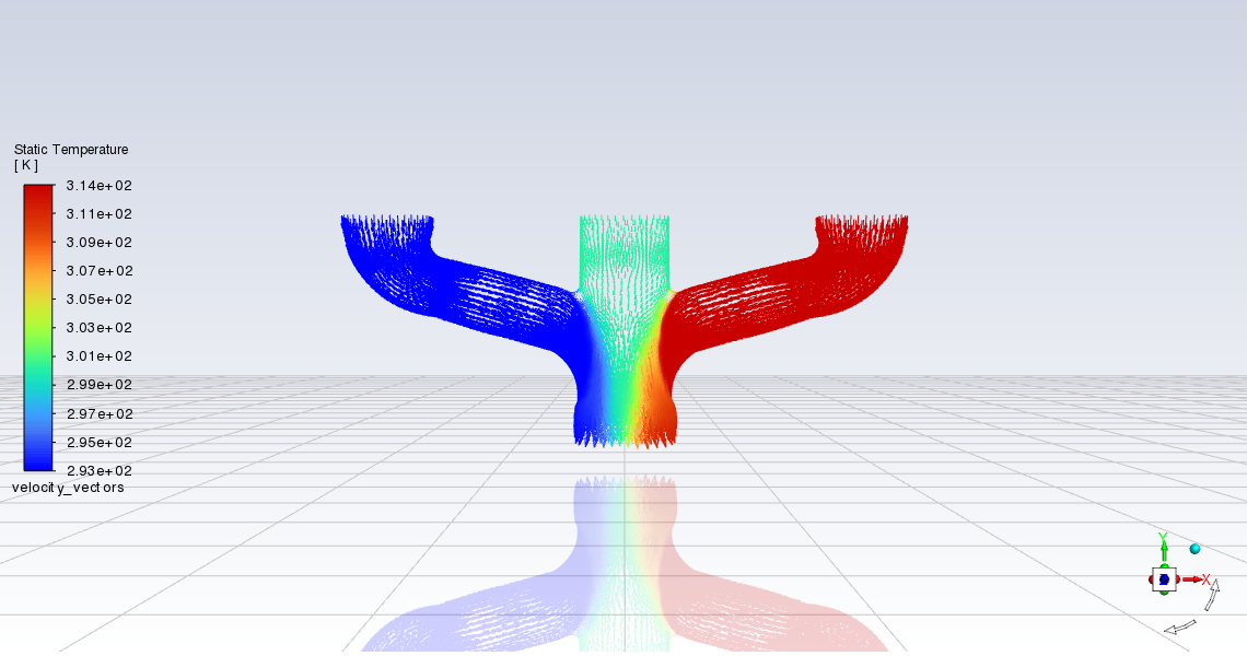
Create and display velocity vectors, colored by temperature:

>>> solver.results.graphics.vector["velocity_vectors"] = {}
>>> solver.results.graphics.vector["velocity_vectors"].field = "temperature"
>>> solver.results.graphics.vector["velocity_vectors"].surfaces_list = ["in*", "out*", "solid*"]
>>> solver.results.graphics.vector["velocity_vectors"].scale.scale_f = 4
>>> solver.results.graphics.vector["velocity_vectors"].style = "arrow"
>>> solver.results.graphics.vector["velocity_vectors"].display()

Figure 32.3: Velocity Vectors Colored by Temperature

Compute the mass flow rate.

>>> solver.solution.report_definitions.flux["mass_flow_rate"] = {}
>>> solver.solution.report_definitions.flux["mass_flow_rate"].boundaries = ["velo*", "pres*"]
>>> solver.solution.report_definitions.flux["mass_flow_rate"].print_state()
>>> solver.solution.report_definitions.compute(report_defs=["mass_flow_rate"])

The output is:

      mass_flow_rate
 -------------------
                  Mass Flow Rate              [kg/s]
-------------------------------- -------------------
                  mass_flow_rate       6.9705571e-05
[{'mass_flow_rate': [6.970557133634259e-05, 0]}]

Close Fluent
```
>>> exit()
```