


FFT PSF

Computes the diffraction point spread function (PSF) using the Fast Fourier Transform (FFT) method.
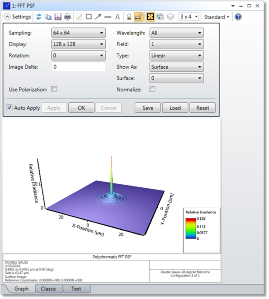
Sampling The size of the ray grid used to sample the pupil. The sampling may be 32x32, 64x64, etc. Although higher sampling yields more accurate data, calculation times increase.
Display The display size indicates what portion of the computed data will be drawn when a graphic display is generated. The display grid can be any size from 32 x 32 up to twice the sampling grid size. Smaller display sizes will show less data, but at higher magnification for better visibility. This control has no effect on the text display.
Rotation Rotation specifies how the surface plots are rotated for viewing; either 0, 90, 180, or 270 degrees.
Wavelength The wavelength number to be used in the calculation.
Field The field number for which the calculation should be performed.
Type Select linear (intensity), logarithmic (intensity), phase, real part (signed amplitude), or imaginary part (signed amplitude).
Show As Choose surface plot, contour map, grey scale, or false color map as the display option.
Use Polarization if checked, polarization is considered. See "Polarization (system explorer)" for information on defining the polarization state and how polarization is used by analysis features.
Image Delta The delta distance between points in image space, measured in micrometers. If zero, a default spacing is used. If negative, the image delta is set to the maximum allowed value and the full sampling grid is used. See the discussion for details.
Normalize If checked, the peak intensity will be normalized to unity. Otherwise, the peak intensity is normalized to the peak of the unaberrated PSF (the Strehl ratio).
Surface Selects the surface at which the PSF is to be evaluated. This is useful for evaluating intermediate images. See "Evaluating results at intermediate surfaces".
Discussion
The FFT method of computing the PSF is very fast, however, a few assumptions are made which are not always valid. The slower, but more general Huygens method makes fewer assumptions, and is described in "Huygens PSF"
Assumptions used in the FFT PSF calculation
The FFT PSF computes the intensity of the diffraction image formed by the optical system for a single point source in the field. The intensity is computed on an imaginary plane which is centered on and lies perpendicular to the incident chief ray at the reference wavelength. The reference wavelength is the primary wavelength for polychromatic computations, or the wavelength being used for monochromatic calculations. Because the imaginary plane lies normal to the chief ray, and not the image surface, the FFT PSF computes overly optimistic (a smaller PSF) results when the chief ray angle of incidence is not zero. This is often the case for systems with tilted image surfaces, wide angle systems, systems with aberrated exit pupils, or systems far from the telecentric condition.
The other main assumption the FFT method makes is that the image surface lies in the far field of the optical beam. This means the computed PSF is only accurate if the image surface is fairly close to the geometric focus for all rays; or put another way, that the transverse ray aberrations are not too large. There is no hard and fast limit, however if the transverse aberrations exceed a few hundred wavelengths, the computation is likely not accurate. Note that even systems with very little wavefront aberration can have large transverse ray aberrations; for example, a cylinder lens which only focuses rays along one direction. In this case, the transverse aberrations along the unfocused direction will be on the order of the beam diameter. The Huygens PSF method may provide more accurate results in these cases as well.
For most lenses, a less important assumption is that scalar diffraction theory applies. The vectorial nature of the light is not accounted for. This is significant in systems that are very fast, around F/1.5 (in air) or faster. The scalar theory predicts overly optimistic (a smaller PSF) results when the F/# is very fast.
For systems where the chief ray is nearly normal (less than perhaps 20 degrees), the exit pupil aberrations are negligible, and the transverse ray aberrations are reasonable, then the FFT PSF is accurate and generally much faster than the Huygens PSF method.
When in doubt, both PSF methods should be employed for comparison. A solid understanding on the part of the user of these assumptions and the method of computation is essential to recognize cases where the accuracy may be compromised.
Discussion of the FFT method and sampling issues
The FFT PSF algorithm exploits the fact that the diffraction PSF is related to the Fourier transform of the complex amplitude of the wavefront in the exit pupil of the optical system. The amplitude and phase in the exit pupil are computed for a grid of rays, an FFT is performed, and the diffraction image intensity is computed.
There is a tradeoff between the sampling grid size in the pupil, and the sampling period in the diffraction image. For example, to decrease the sampling period in the diffraction image, the sampling period in the pupil must increase. This is done by "stretching" the pupil sampling grid so that it overfills the pupil. This process means fewer points actually lie within the pupil.
As the sampling grid size is increased, OpticStudio scales the grid on the pupil to yield an increase in the number of points that lie on the pupil, while simultaneously yielding closer sampling in the diffraction image. Each time the grid size is doubled, the pupil sampling period (the distance between points in the pupil) decreases by the square root of 2 in each dimension, the image surface sampling period also decreases by the square root of 2 in each dimension, and the width of the diffraction image grid increases by a factor of the square root of 2 (since there are twice as many points in each dimension). All ratios are approximate, and asymptotically correct for large grids.
The stretching is referenced to a grid size of 32 x 32. The 32 x 32 grid of points is placed over the pupil, and the points that lie within the pupil are actually traced. For this grid size, the default distance between points in the diffraction image surface is given by

where F is the working F/# (not the same as the image space F/#), is the shortest defined wavelength, and n is the number of points across the grid. The -2 factor is due to the fact the pupil is not centered on the grid (since n is even), but is offset at n/2 + 1. The 2n in the denominator is due to the zero-padding described later.
For grids larger than 32 x 32, the grid is by default stretched in pupil space by a factor of  each time the sampling density doubles. The general formula for the sampling in image space is then

and the total width of the image data grid is

Since the stretching of the pupil grid decreases the number of sample points in the pupil, the effective grid size (the size of the grid that actually represents traced rays) is smaller than the sampling grid. The effective grid size increases as the sampling increases, but not as quickly. The following table summarizes the approximate effective grid size for various sampling density values.
DEFAULT EFFECTIVE GRID SIZES FOR PSF CALCULATIONS
| Sampling Grid Size | Approximate Effective Pupil Sampling |
| 32 x 32 | 32 x 32 |
| 64 x 64 | 45 x 45 |
| 128 x 128 | 64 x 64 |
| 256 x 256 | 90 x 90 |
| 512 x 512 | 128 x 128 |
| 1024 x 1024 | 181 x 181 |
| 2048 x 2048 | 256 x 256 |
| 4096 x 4096 | 362 x 362 |
| 8192 x 8192 | 512 x 512 |
The sampling is also a function of wavelength. The discussion above is only valid for the shortest wavelength used in the calculation. If the computation is polychromatic, then the longer wavelengths will be scaled to have smaller effective grids. The scale factor used is the ratio of the wavelengths. This should be considered when selecting sampling grids for systems with broad wavelength bands. For polychromatic computations, the data for shorter wavelengths is more accurate than for longer wavelengths. For the FFT PSF phase, real, and imaginary data types, the polychromatic average is not physically meaningful, and OpticStudio will set the wavelength selection to the primary wavelength if the user selected all wavelengths.
The image delta, Δ, can be selected manually if a different sampling distance is required. If the image delta is zero, OpticStudio uses the default spacing and sampling grids described above. If the image delta is greater than zero, then OpticStudio scales the pupil sampling to yield the desired image delta size. The actual amount of stretching depends upon the grid size, the image delta, the defined wavelengths, the F/#'s at each field and wavelength, and the aspect ratio of the exit pupil. If the image delta is set too small, then not enough points will be left to sample the pupil; if the image delta is too big, then the pupil grid will not extend over the full width of the exit pupil. Both of these cases are trapped by OpticStudio and an error message will be issued if they occur. If the image delta is less than zero, then OpticStudio does not stretch the pupil at all. This maximizes the extent of the PSF in image coordinates and uses the full grid of rays in the pupil, at the expense of not increasing the spatial resolution with sampling, as the image delta will be nearly constant with increased sampling.
Once the sampling is specified, OpticStudio doubles the array size in a process called "zero padding". This means for a 32 x 32 sampling, OpticStudio uses the center portion of a 64 x 64 grid. Therefore, the diffraction PSF will be distributed over a 64 x 64 size grid. The sampling in the image space is always twice the pupil sampling. Zero padding is performed to reduce aliasing.
The nature of the FFT algorithm is that the computation is done in pupil space coordinates. For this reason, rotating the image surface will have no effect on the orientation of the computed PSF. The X and Y orientation of the PSF corresponds to the X and Y orientation of rays in the entrance pupil, which is not always the same as the spatial X and Y orientation of the image. To compute the PSF in the image space coordinates, see "Huygens PSF"
Next: