Available Scatter Models

There are seven scattering models available: none, Lambertian, Gaussian, ABg, ABg File, BSDF, and user defined.

Each available scatter model is defined in the following sections.

No Scattering

No modification to the specular ray is made, the BSDF is zero and the magnitude of the vector is zero.

Lambertian Scattering

For Lambertian scatter, the scattered ray projection vector has equal probability anywhere in the unit circle, and the BSDF is just 1/π .

The scattered intensity is proportional to cos θ_s.

Note Lambertian scattering is independent of the ray incident angle. Most diffuse surfaces are nearly Lambertian.

Gaussian scattering

Gaussian scattering is of the form:

where A is a normalizing constant. The resulting distribution is rotationally symmetric in direction cosine space, no matter what angle the specular ray makes with respect to the surface normal. The dimensionless value σ determines the width of the Gaussian distribution on the projected plane. Values of σ greater than about 5.0 yield a BSDF that is nearly Lambertian. For this reason, the maximum allowed value of σ is 5.0.

ABg Model Scattering

The ABg scattering model is a widely used method for defining the BSDF. This scattering model is generally a good model to use when the scattering is mainly due to random isotropic surface roughness, and the scale of the roughness is small compared to wavelength of light being scattered. These assumptions are generally valid for polished optical surfaces. The ABg BSDF is given by

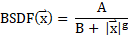
The following restrictions are placed on the coefficients of this model:

A must be greater than or equal to 0.0, and B must be greater than 1E-12 unless g = 0.0.

If g is 0.0, B may be 0.0.

If A is 0.0, no scattering will occur.

If g is 0.0 (note g may be any value, positive or negative, but it typically is between 0.0 and 3.0), then the BSDF is constant:

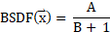
and the resulting scattering is effectively Lambertian.

For highly polished surfaces (especially when g >> 1.5 and B << 1E-8), the amount of power scattering into diffuse angles will be negligible in comparison to the specular power. The consequence of this is that OpticStudio will not accurately resolve the scattered power at large angles. This is due to a numerical limitation for systems with very highly polished surfaces.

If A, B, and g are set to provide a relatively flat BSDF curve, it is far faster numerically to use the Lambertian model instead.

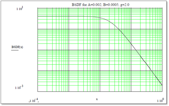
A typical ABg BSDF curve is shown below for the parameters A = 0.002, B = 0.0005, g = 2.0.

The ABg BSDF model has several interesting properties (when g is not zero):

When the BSDF curve flattens out to a value of A/B as goes to zero.

When the BSDF becomes a straight line on the log-log plot, with a slope of -g.

The transition point between the flat and sloped parts of the curve occurs at where

Defining ABg data

It is frequently the case where the same ABg data will be applied to many objects in the optical system. To avoid the need to type in the same data redundantly, and to simplify the task of editing the ABg data, OpticStudio provides an ABg data catalog. The catalog may be edited directly in OpticStudio; see "ABg Scatter Data Catalogs". Note the ABg data defined must integrate over all possible scatter angles to a total value of less than 1.0 to conserve energy.

OpticStudio allows definition of separate ABg data for reflection and refraction. If the specular ray reflects or refracts, the ray is subsequently scattered using the appropriate coefficients. The ABg data names which appear in the dialog box control are those defined by the ABg scatter data file. The ABg data file to be used is selected from the "Files" section of the System Explorer.

OpticStudio first decides whether or not to scatter the ray, as described in the section "Scattering" above. If the ray scatters, a scattered ray is randomly generated. The ray direction is generated so that if a large number of rays were scattered, the appropriate BSDF function would result.

For important information on using scatter models with a source defined by a Source Color spectrum, see "Wavelength scaling of ABg data".

ABg File Scattering

The ABg File scattering model allows a sum of ABg profiles to be used to define the scattering properties of a surface. The profiles to use are specified in a text file. The text file must have a .ABGF extension and must be located in the <data>\ABg_Data folder (see "Folders"). All of the profiles specified in the ABGF file must be defined in the currently loaded ABg Data File (see "ABg Data File"), and all profiles must be specified using upper case letters (regardless of capitalization of the profile name in the ABg Data File).

The syntax of the ABGF file is:

 
Number of profiles Weights_Are_Absolute<optional> Profile_1_Name Profile_1_Weight
Profile_2_Name Profile_2_Weight
...

The first line of the file should contain either 1 or 2 numbers: the first defining the number of ABg profiles contained in the ABGF file, and the second (optional value) defining a flag that indicates whether the weights provided for each profile are relative or absolute. If this flag is omitted or set to zero, the profile weights are taken to be relative; otherwise the profile weights are taken to be absolute. In either case, the BSDF values for each profile are multiplied by the corresponding profile weight and then added together. If the profile weights are taken to be relative, the sum of BSDF values is divided by the sum of the weights, and the resulting scatter distribution corresponds to a weighted sum of the defined profiles. Conversely, if the profile weights are taken to be absolute, the sum of the BSDF values is not normalized, and the resulting scattering distribution corresponds to an absolute sum of the profiles. In this latter case, it is up to the user to confirm that the TIS resulting from an absolute sum of the specified ABg profiles does not exceed unity for any wavelength or any angle of incidence.

The remaining lines of the file simply contain the name of each ABg profile to sum and the corresponding weight. The name of the profile should be entered exactly as it appears in the ABg Scatter Data Catalog (see "ABg Scatter Data Catalogs"). Each of the profiles is treated as it would be under the ABg scatter model (see "ABg model scattering"). Thus, ABg data for each profile will be scaled with wavelength if a reference wavelength is defined in the ABg Scatter Data Catalog for that profile, and the ABg data for each profile will be interpolated between the two points with angles of incidence closest to that of the incident angle for the scattered ray. The wavelength scaling and interpolation over angle of incidence will be performed for each profile specified in the ABGF file before all profiles are summed.

The maximum number of profiles which may be specified in an ABGF file is 20. Please contact OpticStudio technical support if you require this limit to be increased.

BSDF Scattering

The BSDF scattering model allows the use of tabular BSDF data for defining the scattering properties of a surface. Data are provided via text files. Files must follow the Zemax Tabular BSDF Data file format described in the article entitled "Zemax Tabular BSDF data file format", check: Zemax Tabular BSDF data file format – Knowledgebase.

OpticStudio allows definition of separate BSDF data for reflection and refraction. If the specular ray reflects or refracts, the ray is subsequently scattered using data from the appropriate input file. For a file to be available for use in this scatter model, it must have a .BSDF extension (as indicated in the article describing the file format), and be located in the <data>\Scatterdata folder (see "Folders"). The maximum number of characters that the file name can contain (including the .BSDF extension) is 60.

A full description of the model and its use is provided in the Knowledge Base article entitled "How to Use Tabular Data to Define the Surface Scattering Distribution" (See: How to use tabular BSDF data to define the surface scattering distribution – Knowledgebase (zemax.com)) also available on the OpticStudio web site.

User Defined Scattering

Completely general surface scattering may be defined via an external program called a Dynamic Link Library (DLL). Sample DLLs are provided with OpticStudio with source code. New DLLs may be easily created with a suitable compiler. See also "Comments about DLLs".

Defining an Object to use DLL Defined Surface Scattering

To make an object use a DLL defined scatter function, choose the "User Defined" scattering type from the object properties dialog box, then select from the available DLL scatter functions listed in the "DLL Name" box.

To check the input and output data for each DLL, check: Data[] values for Bulk Scatter, Diffraction, Surface Scatter DLLs.

DLL parameters

Each DLL may use up to 6 user defined data values as parameters in the computation of the scattering properties. These values are defined by the DLL and are only used by the DLL.

Creating a new DLL

The DLL must include two functions:

• UserScatterDefinition
• UserParamNames

When a ray is scattered, OpticStudio passes to the UserScatterDefinition function the local x, y, and z coordinates on the surface, the local normal vector, the local specular ray vector, polarization data, and other parameter data as defined by the user.

UserScatterDefinition then is required to determine the following values:

• Whether or not the ray actually scatters
• The direction cosines of the scattered ray
• The attenuation of the ray, if any
• Optionally the new electric field vector (if this is not provided OpticStudio will make a reasonable guess)
• Optionally the BSDF and TIS if Importance Sampling is used (see "Importance Sampling")

These values are returned to OpticStudio and are used to continue the trace.

If the new electric field vector is provided, OpticStudio will do an additional check. It will check if the total post-scattering intensity is within 10^-10 of unity. If it is, then OpticStudio considers that this value has been normalized. So OpticStudio will do an adjustment. It will look at the intensity pre-scattering and multiplies each electric field component by the square root of that value in order to un-normalize. This "step" ensures that the electric fields are physical as the intensity can never be that close to 1.

The function UserParamNames is used to define the names of all used parameters. These names appear in the Coating/Scattering tab of the object properties dialog box. Surface scattering DLLs must be placed in the <data>\DLL\SurfaceScatter folder. See "Folders".

Note that the "Fraction to scatter" control is active when User Defined scatter is selected. Only the fraction of energy which is allowed to scatter is sent to the DLL for possible scattering. However, the DLL may choose to not scatter the ray (see for example the sample DLL in the next section).

More details can be found in the source code of the sample surface scattering DLL files provided with OpticStudio.

Sample surface scattering: TwoGaussian.DLL

The surface scattering sample TwoGaussian.DLL supports a scatter model which is the superposition of 4 scattering models: specular, Lambertian, and two individual Gaussian models. The DLL uses the parameter data to define the fraction of energy which scatters according to the Gaussian Sigma 1, the fraction which scatters according to Sigma 2, and the fraction that is Lambertian. The remaining fraction, if any, is specular. To see how this is accomplished in the DLL, review the source code file Two Gaussian.c provided with OpticStudio.

Sample surface scattering: K-correlation.DLL

The surface scattering sample K-correlation.DLL supports a scatter model which follows the K-correlation distribution, as described in the paper "K-correlation power spectral density & surface scatter model" by Michael G. Dittman (Proc. of SPIE Vol. 6291, 62910R, 2006). The inputs to the DLL include the surface roughness (in micrometers), the characteristic surface wavelength (multiplied by 2π ), and the logarithmic slope of the BSDF. More details are provided in the article entitled "How to Model Surface Scattering via the K-correlation Distribution" in the OpticStudio Knowledge Base. The source code K-correlation.c is provided with OpticStudio as a sample file.

Sample surface scattering: RI_BSDF.DLL

The sample RI_BSDF.DLL supports a model in which tabular data are used to define the scattering properties of a surface. This DLL is considered obsolete. Any users wishing to define scattering via tabular input data should use the built-in BSDF scatter model (see "BSDF scattering").

Next:

• Thin Window Scattering