


Sources
Object source options are set in the Source section of the Object Properties window. The Object Properties can be reached by clicking the down arrow in the Object Properties bar above the NSC Editor.
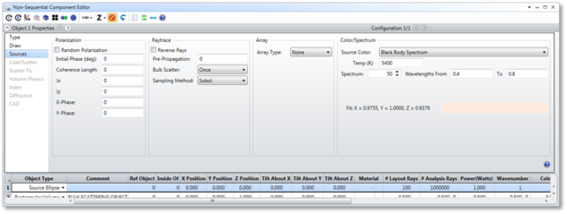
Sources section is used to define properties of source objects, including polarization state, coherence length, and initial phase, position, and direction of rays of light emanating from NSC sources. For important information see "Defining the initial polarization". The tab supports the following controls:
Polarization
Random Polarization If checked, the source will emit randomly polarized light. If unchecked, the polarization state may be defined using other controls in this section.
Initial Phase The initial phase of the ray in degrees, with 360 degrees being equal to one wave of optical path. This setting only affects coherent ray computations which depend upon the phase of the ray.
Coherence Length The length of ray propagation in lens units over which the phase is known. For details on Coherence Length effects see "Coherence length modeling".
Jx, Jy The magnitude of the electric field in the local x and y directions, respectively.
X-Phase, Y-Phase The phase in degrees of the electric field in the local x and y directions, respectively.
Ray Trace
Reverse Rays Checking this option will reverse the direction cosines of every ray. This is useful for reversing the initial direction of rays from the source. Reverse rays is done after the Pre-Propagation distance is considered, if any.
Pre-Propagation The distance in lens units the ray is propagated before beginning the actual ray trace through NSC objects. Pre propagation moves the starting point of rays forward or backward along the ray direction cosines. This feature is useful for defining rays at one position but beginning the ray trace at a different position along the ray path; such as prior to or after an object near the source. The Pre-Propagation distance will alter the initial phase and electric field of the ray to account for the propagation length. Pre-Propagation occurs before reversing the rays if the reverse rays option is selected.
Bulk Scatter Normally, if a ray travels through an object with a bulk scattering media, the rays may scatter multiple times within the media. This is the default "Many" option. If "Once" is selected, each branch of a ray can only bulk scatter once. Note that if a ray splits before scattering, each of the child rays may scatter, since each child's branch is scattering for the first time. If "Never" is selected, then no bulk scattering will occur for rays from this source. This control is useful for modeling fluorescence. See also the "Bulk Scatter" section of the Object Properties.
Sampling Method The available options are random and Sobol. Once the parameters of a source model are defined, rays are generated randomly to model the light leaving the source. However, truly random values are not always desirable. The reason is that random numbers tend to not uniformly sample parameter space if the number of samples is small. Random numbers may group together, leaving relatively large gaps in sampling space. In practice, this means that it takes a great many rays to get sufficient sampling to produce smoothly varying results. Sobol sampling is a widely used sampling algorithm which looks qualitatively random, but is in fact a carefully selected distribution that optimally "fills in" previously unsampled space. For a discussion of the advantages and disadvantages of random and Sobol sampling, see "Random vs. Sobol sampling".
Array
Array Type This feature creates an array of identical sources, all with the same properties as the "parent" source. Depending upon the Array Type, additional parameters become available on the Source tab to define the number of array elements and the size of the array. The array types supported are:
Rectangular: This array can be used to make a 1D line or 2D array of sources with uniform spacing in the local X and Y directions. The options available include the number of sources in X and Y, and the source to-source spacing in lens units along each direction. The minimum number of sources in either direction is 1, the maximum is 2000. The sources are numbered starting from 1 in the first (x) column and first (y) row at the location of the parent object. Each subsequent source is numbered across the columns along the first row, until the number of x direction sources is reached. The next source will be placed at the next row in the first column, and then numbering continues across the columns again, until all sources are placed.
Circular: This array is a single circle of sources centered on the parent coordinate. The sources are equally spaced in angle at the specified radial coordinate in lens units. The first source is at 0 degrees on the XY plane, and the sources continue counter-clockwise (looking down the -Z axis) around the circle until all sources are placed.
Hexapolar. This array consists of equally spaced rings of sources. The first "ring" is at the location of the parent, and the first source is placed there. The second ring contains 6 sources, equally spaced in angle, starting at source number 2 at +90 degrees on the XY plane, and the sources continue counter-clockwise (looking down the -Z axis) around the circle until all 6 sources (source numbers 2-7) are placed. The third ring contains 12 sources, the fourth ring 18, and the pattern repeats until the last ring is reached. A maximum of 20 rings is supported. The spacing parameter is the radial spacing between adjacent rings.
Hexagonal. This type forms an array with hexagonal symmetry. The first "ring" contains one source at the location of the parent source. The second "ring" contains 6 sources, placed around the center source in hexagonal fashion. The third "ring" consists of 12 sources placed outside of the second ring, and the pattern repeats until the last ring is reached. A maximum of 20 rings is supported. The spacing parameter is the full height of the hexagonal region, which is the vertical spacing between sources in the same column. The numbering convention for this array starts at 1 at the bottom (-y coordinate) of the leftmost (-x coordinate) column, and then goes up the leftmost column, then starts at the bottom of the next column to the right, and proceeds up that column. The pattern repeats until the top source in the right most column is reached.
For all arrays of sources, if the total number of sources exceeds 10,000, the source objects will not be drawn. The parameter settings for the source, such as number of layout rays, number of analysis rays, and power apply to each source in the array. For example, a 3 x 3 array of 1 watt sources will produce 9 watts.
Color/Spectrum
Source Color, Spectrum, and Wavelengths From/To These settings choose the method for generating the spectral model for the source. There are a number of ways to model the spectral content of a source. Sources may be either monochromatic, or may cover some region of the visible spectrum to represent a composite color, such as orange or white. The available source color models are described below.
System Wavelength: If this option is selected, then the monochromatic wavelengths defined on the system wavelength dialog box are used. The system wavelengths are described in "Wavelengths". Once the system wavelengths are defined, the wavelength used for ray tracing is defined by the wavenumber used by the source. The wavenumber is one of the NSC Editor parameters used by all sources. See "Parameters common to all source objects" for a full description. This is the default setting for Source Color and is the only setting that uses the system wavelengths.
CIE 1931 Tristimulus XYZ: This source color model defines the color of the source using the three CIE tristimulus values commonly given the names X, Y, and Z. See "The spectrum fitting algorithm" for important information on the spectrum generated to represent the desired color. Note that although the Y value normally represents the overall brightness of the source in lumens, OpticStudio does not use the Y value for this purpose when defining the source color. The power or brightness of the source is set independently; see "Parameters common to all source objects" for a full description. Internally, OpticStudio will normalize the XYZ values to 1 lumen for purposes of computing the spectrum.
CIE 1931 Chromaticity xy: This source color model is essentially identical to the XYZ model above, except the normalized chromaticity coordinates are used instead. OpticStudio converts the xy values to XYZ and then follows the procedure described in "The spectrum fitting algorithm".
CIE 1931 RGB (Saturated): RGB values are converted to CIE XYZ coordinates, and the method for computing the spectrum is then the same as for CIE 1931 Tristimulus values. Note the RGB color is the fully saturated RGB color, which means colors such as grey on a 8 bit scale (128, 128, 128) are saturated to the maximum brightness (256, 256, 256) and will appear white. There is no difference in the color spectrum of grey and white, or any dark and light colors, as long as the relative color values are maintained.
Uniform Power Spectrum: This creates a uniform power spectrum over the specified wavelength range at the number of discrete wavelengths defined.
D65 White: Defines X = 0.9505, Y = 1.0000, Z = 1.0890, which is the D65 white color on computer monitors.
Color Temperature: Based upon the temperature in Kelvin, the XYZ tristimulus values are computed to yield the same color as a black body of the specified temperature, and the spectrum is computed as described for the CIE 1931 Tristimulus values. Note this is not a true black body spectrum, but a spectrum fit to yield the same color as the blackbody of that temperature.
Black Body Spectrum: Based upon the temperature in Kelvin, this yields a true blackbody spectrum over the specified wavelength range. This color model is not limited to the visible spectrum.
Spectrum File: This color model reads the wavelength values and weights from a file. For details on the file format, see "Defining a spectrum file".
CIE 1976 Chromaticity u' v': This source color model is essentially identical to the XYZ model above, except the normalized u' and v' chromaticity coordinates are used instead. OpticStudio converts the u' and v' values to XYZ and then follows the procedure described in "The spectrum fitting algorithm".
Note that for all Source Color settings other than System Wavelengths, Uniform Power Spectrum, Black Body Spectrum, and Spectrum File, a spectrum must be fit to represent the selected color. See "The spectrum fitting algorithm".
Next: