


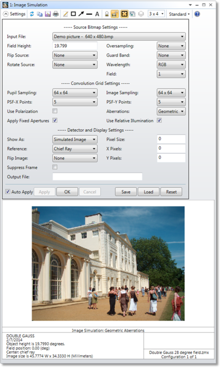
Image Simulation
This feature simulates the formation of images by convolving a source bitmap file with an array of Point Spread Functions. The effects considered include diffraction, aberrations, distortion, relative illumination, image orientation, and polarization.
Source Bitmap Settings
Input File The name of the file for the source bitmap. The file may be in BMP, JPG, PNG, IMA, or BIM file formats. For a description of the IMA and BIM file formats see "The IMA format" and "The BIM format". The input files are stored in the <images> folder (see "Folders" ). IMA abd BIM files must have more than 1 but no more than 8,000 pixels in each direction, while BMP, JPG and PNG files must have more than 1 and no more than 16,000 pixels in each direction.
Field Height This value defines the full height in the y-axis of the source bitmap in field coordinates, which may be either lens units or degrees, depending upon the current field definition (heights or angles, respectively). If the field type is Real Image Height, the field type is automatically changed to Paraxial Image Height for this analysis. This avoids the problem of Real Image Height masking the distortion in the image. The Field Height applies to the resulting bitmap after any oversampling, guard band, or rotation is applied.
Oversampling Oversampling increases the pixel resolution of the source bitmap by copying one pixel into 2, 4, or more identical adjacent pixels. The purpose of this feature is to increase the number of pixels per field unit. Oversampling will be applied a factor of 2 at a time until the specified oversampling is achieved, as long as the maximum number of pixels in any direction will not exceed 16,000. This limit only applies to the oversampling feature, and not to the input file. Oversampling is applied to the image before any effects of the optical system are considered.
Flip Source Flips the source bitmap left-right, top-bottom, or both. The source bitmap is flipped before any effects of the optical system are considered.
Guard Band This feature increases the pixel resolution of the source bitmap by repeatedly doubling the number of pixels. This doubling only affects the analysis, while the original bitmap file remains unchanged. This results in a black "guard band" all around the original image. The purpose of this feature is to increase the number of pixels per field unit while adding a region around the desired image. This is particularly useful if the point spread function(s) are large compared to the source bitmap field size. The guard band will be applied a factor of 2 at a time until the specified size is achieved, as long as the maximum number of pixels in any direction will not exceed 16,000. This limit only applies to the guard band feature, and not to the input file. The guard band is applied to the source bitmap before any effects of the optical system are considered.
Rotate Source Rotates the source bitmap. The rotation is applied to the source bitmap before any effects of the optical system are considered.
Wavelength If "RGB" is selected, then 3 wavelengths will be defined, 0.606, 0.535, and 0.465 micrometers for red green, and blue, respectively; no matter what the current wavelength definitions are. If "1+2+3" is selected, then wavelengths 1, 2, and 3 as currently defined on the wavelength data box will be used. The red channel of the source bitmap will be used for wavelength 3, green channel for wavelength 2, and the blue channel for wavelength 1. The displayed image will be in RGB format no matter what wavelengths are defined using this option. For selection of a specific single wavelength, such as 6, the B channel image will be used for wavelengths 4, 7, 10, 13, etc. The G channel image will be used for wavelengths 5, 8, 11, 14, etc. The R channel image will be used for wavelengths 6, 9, 12, 15, etc.
Wavelength weighting is usually ignored. The color weighting that results in the final image depends only upon the color amplitude in the source bitmap and the relative transmission of the optical system. The exception is when using monochromatic IMA files, the selected wavelength is "1+2+3", and 3 wavelengths are defined. In this case only, the wavelength weighting is used to define the relative color weighting.
Field The source bitmap may be centered on any defined field position. The resulting image is then centered on this field position.
Convolution Grid Settings
Pupil Sampling The grid sampling to use in the pupil space for computing the PSF grid.
Image Sampling The grid sampling to use in the source bitmap space for computing the PSF grid.
PSF X/Y Points The number of field points in the X/Y direction at which to compute the PSF. For field points in between these grid points, an interpolated PSF is used.
Use Polarization If checked, polarization is considered. See "Polarization (system explorer)" for information on defining the polarization state and how polarization is used by analysis features.
Apply Fixed Apertures If checked, all surfaces with optical power that have no aperture defined are modified for this computation to have a circular aperture at the current clear semi-diameter or semi-diameter value. Without this change in the aperture definition, rays may pass the surface beyond the listed clear semi-diameter or semi-diameter, especially if the Field Height exceeds the field of view defined by the field points. This leads to misleading illumination, typically at the edges of the image.
Use Relative Illumination If checked, then the computation described in "Relative Illumination" is used to weight the rays from various points in the field of view to accurately account for the effects of exit pupil radiance and solid angle. The computation is generally more accurate, but slower, if this feature is used. Note that if there are too few rays that can trace through the system to image surface, relative illumination is considered as zero and the result can be inaccurate. Users can check the result whether this happens by using the analysis Relative Illumination with default settings. If unchecked, then the calculation uses the chief ray to establish the overall intensity. Note if the chief ray cannot be traced, the relative illumination is considered as zero when this option is unchecked. If the chief ray isn't traceable, try checking "Use Relative Illumination".
Aberrations Choose None to ignore aberrations, Geometric to consider only ray aberrations, or Diffraction to use the Huygens PSF to model the aberrations. If Diffraction is selected, the analysis may automatically switch to Geometric if the aberrations are so severe that the diffraction PSF cannot accurately be computed. See the discussion below.
Detector and Display Settings
Show As Choose Simulated Image, Source Bitmap to see the input bitmap (including the effects of oversampling, guard band, and rotation), or PSF Grid to see all of the PSF functions computed over the field of view. See the discussion below.
Reference Selects the reference coordinate for the center of the plot: chief ray, surface vertex, or primary wavelength chief ray. The latter option chooses the primary wavelength chief ray even if some other wavelength is the only one selected.
Suppress Frame If checked, the frame is not drawn and the entire window is used to display the image.
X/Y Pixels The number of pixels to use in the detected image. Use 0 for the default value, which is the number of pixels in the source bitmap.
Pixel Size The simulated image pixel size (square). For focal systems, the units are lens units. For afocal systems, the units are cosines. Use 0 for the default value, which is computed from the magnification of the optical system for the center pixel in the source bitmap. Note that the default-value computation is purely ray-based; if the Field Height is small enough such that the geometric image is smaller than the PSF, this results in an unreasonably small pixel/detector size.
Flip Image Flips the simulated image left-right, top-bottom, or both.
Output File If a file name ending in the BMP, JPG, or PNG extension is provided, then the simulated image will be saved in the specified file and be placed in the <images> folder (see "Folders").
Discussion:
The Image Simulation algorithm consists of the following steps to compute the appearance of the image.
- The source bitmap is oversampled, rotated, and a guard band is applied, if these options are selected.
- A "grid" of Point Spread Functions (PSFs) are computed. The grid spans the field size, and describes the aberrations at selected points in the field of view defined by the bitmap and field size settings. The PSF grid also includes the effects of polarization and relative illumination.
- The PSF grid is interpolated for every pixel in the modified source bitmap. At each pixel, the effective PSFis convolved with the modified source bitmap to determine the aberrated bitmap image.
- The resulting image bitmap is then scaled and stretched to account for the detected image pixel size, geometric distortion, and lateral color aberrations.
The most important part of the algorithm is the computation of the PSF grid. The PSF X/Y Points settings determine how many PSFs are computed in each direction over the field of view. There are three different methods for modeling the aberrations using the PSF: Diffraction, Geometric, and None. Diffraction uses the Huygens PSF (for details see "Huygens PSF").
The Huygens PSF accurately models diffraction effects for almost any optical system, but is slower than the Geometric PSF, which is based upon an integration of the Spot Diagram. The Huygens PSF also cannot be accurately computed if the aberrations are severe (for this feature, the threshold is 20 times the diffraction limit). The Image Simulation algorithm detects when the Huygens PSF cannot be computed, and will automatically switch to the Geometric PSF if required. This switching is done independently for each field and wavelength, and so imaging systems that are diffraction limited in one part of the field but severely aberrated in other parts of the field can still be accurately modeled if Diffraction is selected. If None is selected for the aberration type, the PSF grid is an array of delta functions and aberrations other than lateral color and distortion are not considered.
Relative illumination and (optionally) polarization are considered in the PSF computation. The PSF Grid is smoothly interpolated between computed field points to estimate the PSF at each pixel in the modified source bitmap. The resulting PSF is then convolved with the source bitmap to yield the aberrated image. The more PSF grid points that are used, the more accurate the simulation is, but the longer the computation time.
If the image surface is not a plane, the aberrations and distortion are all computed on the curved image surface, and the Simulated Image is projected onto the XY plane, ignoring the z coordinate of the image surface. The pixels are assumed to be square on the projected plane.
The brightness of the output image is determined by normalizing the image to have the same peak brightness as the input image. If "Use Relative Illumination" is not checked, then the chief ray has to be traceable in order to establish a relative illumination across the image.
The simulated image is shown as it would appear when viewed looking down the local negative Z axis of the image plane.
Default Pixel Size and Image Size
If the parameter Pixel Size is set to 0, the default value is calculated in following way.
- Calculate pixel size at field space, which is (Field Height)/(Bitmap Y Pixels). Note the unit of pixel size at field space depends on the Field Type.
- Trace rays from upper-right and lower-left corners of the center pixel at field space, and get the rays' coordinates at image plane.
- The default pixel size at image plane is then calculated from the rays' coordinates at image plane as shown in following figure.
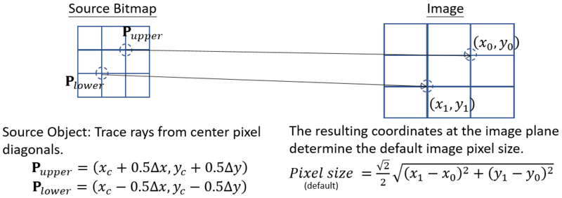
where xc and yc are field coordinate defined by Field in the setting, ∆x and ∆y are the pixel size calculated in step 1.
The Image Size shown at the bottom text in Image Simulation result is then the product of pixel size and pixel numbers in x and y directions. See the explanation for X/Y Pixels for pixel numbers in x and y.
Suggestions for use
The accuracy of the simulation is always ultimately limited by the resolution of the input image. If the resolution of the optical system is sufficient, the discrete pixel nature of the source bitmap may be apparent. This can be manifested by stair-case like edges in the simulated image. The oversampling feature can reduce these effects at the expense of longer computation time.
If the field of view is large, it is often the case that the PSFs are small compared to the area of a single pixel. In this case, a lot of computation of the PSF may yield what is effectively a delta function, with only a single pixel representing the entire PSF. The computation can be done much faster in these cases by ignoring aberrations, or at least by switching from diffraction to geometric PSF computations.
If the magnification or field of view are small enough to yield an image that is comparable in size to the PSF, or perhaps even smaller than the PSF, then the Guard Band feature is likely required. The reason is that the PSF convolution is done over the source image pixels. If the PSF is larger than the source bitmap in image space, the convolution loses the "spread" outside the original bitmap caused by the large PSF. The guard band adds a black region around the original image which can be used to show the spread due to the PSF.
By far the most important diagnostic is the "PSF Grid" under the "Show As" setting. It is always a good idea to look at the PSF grid, and confirm it shows well sampled data, before computing the Simulated Image.
Comments on using field angles
The Field Height determines the physical size of the source bitmap as seen by the optical system. For example, if a 30 x 30 pixel source bitmap is used, and the Field Height is 2.0 mm (this assumes the fields are defined in terms of object heights), then each pixel represents a 66.67 micrometer region. If the same source bitmap is later used with a system with a 40 degree full field of view (using field angles), then the Field Height can be set to 40 to cover the entire field. Each pixel will now represent a 1.33 degree square. The difficulty in using field angle for defining the object field of view is that field angle units are inherently anamorphic. X-direction angles represent a different subtended angle at a Y angle of 80 degrees than at an a Y angle of 10 degrees. If field angles are being used, and the field of view is fairly wide (more than about 40 degrees in any direction) then great care should be taken in interpreting the results for an extended object.
For a precise definition of the field angles OpticStudio uses, see "Field angles and heights".
Comments on using paraxial and real image height
Note that if fields are defined by image height, then Field Height determines the size of the object in image space, not object space. The Field Height is always in whatever units the fields are defined in, and so when using image height as a field type the Field Height determines the source bitmap height in image space. The size of the source in object space is then determined by the Field Height divided by the magnification of the lens.
When using paraxial image height, the anamorphic magnification of the system (if any) will be masked in the simulated image. When using real image height, all forms of distortion will be masked. For this reason, this feature will use paraxial image height for the field definition even if real image height is selected.
However, it is recommended that neither real nor paraxial image height be used. Instead, use object height for finite conjugate systems or field angle for infinite conjugate systems, as these field types unambiguously define the size and orientation of the object in image space.
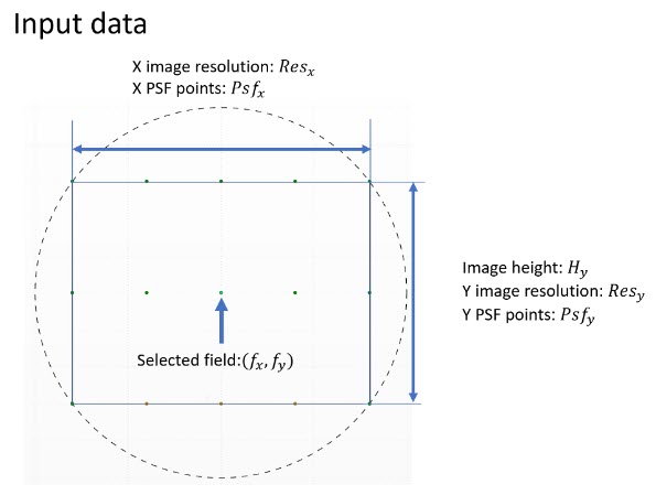
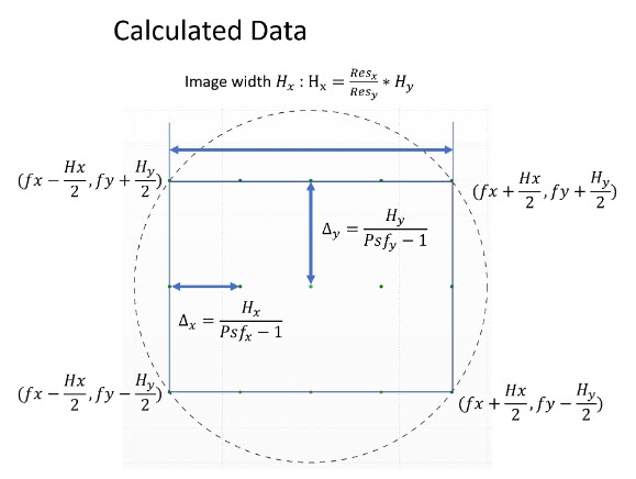
The PSF grid is generated from the object side. It is like the grid distribution type in Fields Wizard. The difference is that the minimum value of pixel number is 1 and the coordinate of the center is half of the resolution. When calculating the PSF's at each grid point, the PSF is centered on the chief ray for the field at that grid point.
The data required to generate the PSF gird are:
Comments on distortion
The distortion algorithm in the Image Simulation depends in part on tracing parabasal rays and in cases where a central obscuration is present, the distortion model may produce non-physical results. Also, the algorithm of distortion can generate some non-physical artifacts at or very near to 90-degree field angle when the object is at infinity, which means afocal in object space. Use the Geometric Bitmap Image Analysis to cross-check that the distortion is correctly calculated in situations where a central obscuration is present.
Next: