Viewing Transient Response Plot
- Open the Signal Net Analyzer.
- Use the Display drop-down menu to select Transient Response Plot.
- Use the Ctrl or Shift keys to click a path in the plot area.
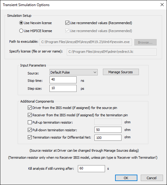
- Click Transient Simulation Options to open the Transient Simulation Options window.
- Configure the settings as appropriate.
- Select either Nexxim or HSPICE, and the paths to both the executable file and license.
- From the Input Parameters area, select an input source. Click Manage Sources to add or delete sources.
- Enter a Stop time and Step size.
- From the Additional Components area, check all appropriate options. Specify ohm values if appropriate.
- From the Kill Analysis if still running after field, specify the maximum time you want to try to run the analysis. The analysis will abort after the time specified.
- Click OK.
- Click Compute Plot.
- To perform transient analysis in bulk (superimpose and compare plots), check the Accumulate Selections for Transient Analysis check box.
- To manually reverse a net path, check the Reverse Selected Path for Transient Analysis check box.
- To run the analysis in Ansys Electronics Desktop, check the Run Transient Analysis in Ansys Electronics Desktop check box. SIwave displays the netlist for the W-element, and Ansys Electronics Desktop opens to run the transient analysis and display the resulting time domain plots.
- To simulate each leg of a differential pair separately, check the Split Differential Nets check box. SIwave lists the positive and negative nets as individual single-ended rows in the grid. Metrics, such as skew and delay, can be examined independently. This option overrides the default behavior where selecting one leg of a differential pair automatically loads the full pair. Use this option to avoid having to delete the differential net definition in the project file when analyzing single-ended behavior.