Field Overlay and Animation
In thermal analyses, field overlays provide a visual indication of temperature and heat flux results, each of which can be overlaid on selected objects or faces:
The available predefined thermal field overlay results are listed and described under Field Overlay in the Results (Thermal) topic. Examples of 2D plots, Stacked plots, and Data Tables follow:
To Produce a Field Overlay Plot and Animate it:
- Select the Faces or Objects on which you want to overlay thermal results.
- Access the Create Field Plot dialog box using one of the following three methods:
- Using the menu bar, click IcepakFEA > Fields > Plot Fields > desired result.
- Right-click Field Overlays in the Project Manager and choose Plot Fields > desired result from the shortcut menu.
- Right-click in the Modeler window and choose Plot Fields > desired result.
- If you selected Named Expression in the previous step, click the desired named expression in the Selecting calculated expression dialog box that appears. Then, click OK.
- In the Create Field Plot dialog box that appears, select the desired setup from the Solution drop-down menu (if you solved more than one analysis setup).
- Optionally, if solid objects were selected for the overlay (as opposed to faces), you can clear the Plot on surface only option to view temperatures and heat flux magnitudes that occur in the interior of the solid objects.
- Click Done.
- Optionally, double-click the plot legend to access and modify the plot properties (scale, color map, and so on).
- If your solution has multiple sets of field results (such as when you run a transient solution or a parametric analysis to vary a design parameter), you can animate your thermal field results.
- Under Field Overlays in the Project Manager, right-click your field overlay and choose Animate from the shortcut menu.
- Optionally, change the Name and/or type a Description for the animation setup.
- Using the two drop-down menus in the Swept Variable(s) tab, choose the setup or variable you want to use as the basis of the animation.
- If you want to base the animation on a single design variable, choose Single Variable and the variable name.
- If you want to base the animation on a parametric setup, choose Parametric Setup and the parametric setup name.
- For transient solutions, choose the start, stop and step values in time units.
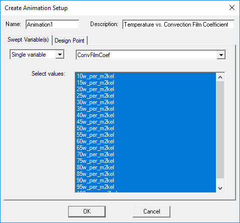
- When applicable, select the variations you want to include in the animation.
- Click OK.
- Use the animation controls to stop, restart, reverse, increase/decrease the speed, or to go to a particular animation frame.
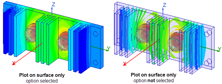
When this option is selected, the results are rendered on the model surfaces only. If you clear this option, the results are rendered for the full model volume, but they are rendered as IsoValSurfaces. Rather than the full volume of the model being rendered in varying colors, IsoValSurfaces connect points of the same resultant value and are rendered for each scale division specified in the plot settings (15 values by default). This plot style enables you to see the results on the interior of solids without creating clipping planes. The following heat sink temperature images compare the two plot styles:
The following field plot setup example produces the heat flux vectors throughout the volume of the selected object or objects:
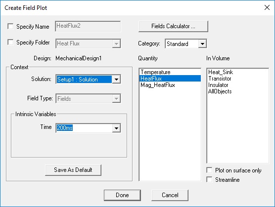
Choices appear in the Intrinsics section only if multiple variants or timesteps are available for plotting (for example, in parametric or transient analyses).
The overlay and result legend appear on the model in the Modeler window.
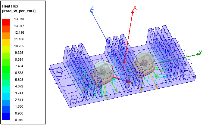
The following image is a HeatFlux (vector) overlay. The legend's number format and units (W/cm2) have been customized:
The Create Animation Setup dialog box appears. However, if your solution lacks multiple field result sets, an error message will appear indicating that the overlay cannot be animated.
For example:
The following example shows the setup for a 10 second transient solution with a timestep size of 0.2 seconds and every step saved:
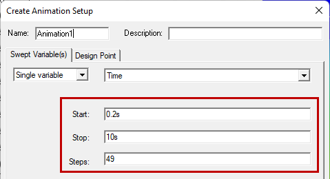
For transient solutions, you must choose the Start, Stop, and Steps values carefully. If the time values determined for every step do not correlate with the time values of the actual transient solution timesteps, blank overlays will occur for the animation frames. Also, remember to subtract 1 from the number of timesteps or animation frames to get the correct number of Steps.
The Start, Stop, and Steps values are filled in automatically when you create an animation setup. The default is to include all available timesteps as an animation frame. If you later adjust the solution's transient setup and rerun it, the animation setup values will not be updated. In this case, the easiest solution is to delete the old animation setup and create a new one.
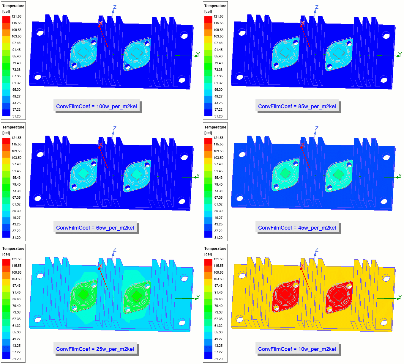
The following example shows all variations of a convection film coefficient variable (ConvFilmCoef) selected.
The Animation dialog box appears and the overlaid results are animated.
An animation based on the preceding parametric example is shown below. The animation was reversed (to progress from the greatest to the smallest convection film coefficient) to show the frames in order of increasing temperature: