Shell Elements Theory

Layered Impedance Boundaries include an option to designate two-sided boundaries as shell elements. For Finite Conductivity boundaries, if DC thickness is set and the user selects two-sided, they can also designate that the boundary be treated as a shell element. If the layered structure is within a 3D model, meshing thin layers and solving inside may be inefficient, so replace the highly conductive thin layer with a shell element. The Shell Element option only applies to HFSS Driven solution types and does not apply to HFSS Eigenmode and Transient solution types. Shell elements are useful for both shielding and radome applications. They can touch or intersect other boundary conditions or materials. They must be valid across a broad frequency range. Example uses include simulation of an antenna inside a car chassis or an antenna inside a dielectric radome, when the chassis and/or radome is modeled using sheets. Shell elements maintain two sets of unknown coefficients for the top and bottom surface.

HFSS uses non-classical shell elements. Classical shell elements appear as prism elements created by doubling tangential components of the electrical field on both sides of a layer. This assumes constant linear or higher order variation in the normal direction. This classical approach is limited in application when the layer is not thin enough to the degree that the field has significant variation in the normal direction or if the field has strong decay in the layer despite it being thin.

Conventional Shell Elements (First Order)

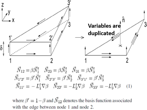
This depicts a degenerated prism element with no 3D mesh assembled on the fly.

Non-Conventional Shell Elements

For non-classical shell elements, we assume that we know the tangential electric and magnetic field on the two sides of the sheet. Rather than evaluate the finite element matrices in the thin prism, we apply a Neuman boundary condition to both sides of the sheet using the circuit Y matrix of the layers. Due to cases where the structure Y matrix cannot be characterized by closed analytical formulas, HFSS uses a two stage method which does not require analytical coupling formulas to replace Frequency Select Surfaces (FSS) by a sheet with shell elements. First, we extract a Y matrix for the FSS by solving a unit cell model of the layer(s). Then we use the Y matrix to couple the two sides of the layer in the FEM. This approach provides accurate and efficient modeling for an arbitrary thin or thick FSS. This is valid for any broad band frequency and material. (See References).

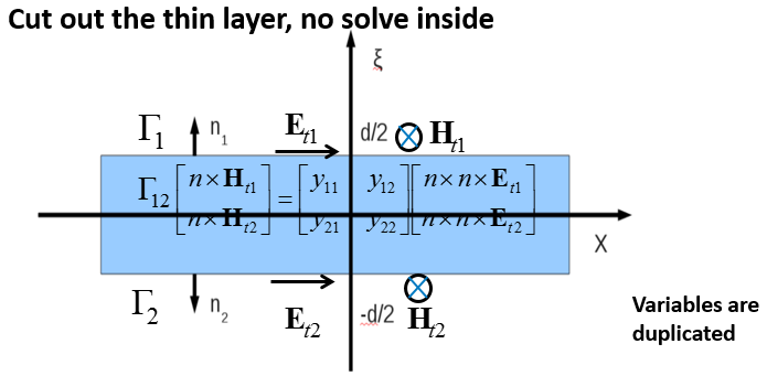
This uses:

• Use a 1D local transmission line model inside
• No Solve Inside, no 3D mesh
• Neumann/natural boundary condition
• Skin effect - copes with strong decay

Conventional versus Non-Conventional Shell Elements

Conventional shell elements:

• accurate
• good for the mesh maker
• can’t cope with strong decay
• higher order is difficult

Non-Conventional shell elements

• approximated by a 1D local model
• good for the mesh maker
• copes with strong decay
• no need for higher order

Finite Element Discretization

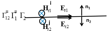
For sheet shell elements, 3D objects are replaced by a sheet:

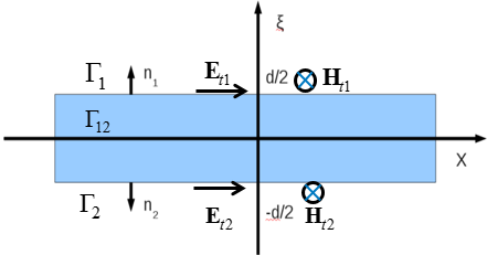
For volumetric shell elements, keep the layer of thickness d, no solve inside.

Finite Element Discretization

Sheet shell elements:

• no mesh inside
• good for the mesh maker
• manual work to get rid of 3D objects

Volumetric shell elements

• good for automation and ease of use
• background mesh inside
• overall mesh quality might be worse

Sheet Shell Elements

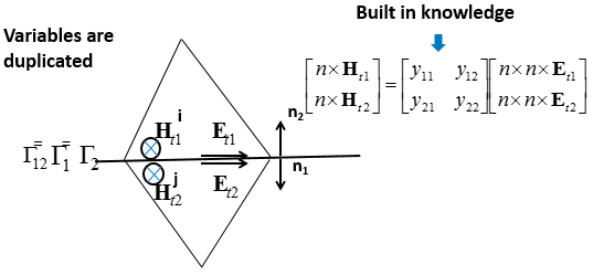
• 3D layer replaced by a sheet
• E DoFs have to be duplicated
• Edges and vertices also can touch the surface

Finite Element Implementation

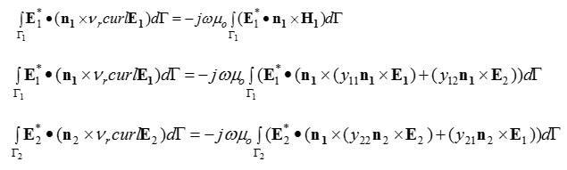
Here E^* denotes weighting functions in the FEM Galerkin method. In this way, a shell element resembles an outer impedance boundary condition. Notice that the field coupling from one side to the other is captured by the term y_ijn_i x E_j in the surface integrals. Furthermore, when assembling a tetrahedron on one side of the sheet, the solver does not include n regular coupling from a tetrahedron on the opposite side except the surface integration contribution just described.

Implementation Issues: Sheet Shell Element Considerations

• Mesh is not modified
• Mesh maker provides the solver with list of shell tets

Implementation Issues: FEM and Sheet Shell Elements

Broad frequency range: Singlar matrix at low frequencies when E tangential components are continuous.

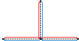
Boundary edges always have impedance:

Intersecting edges:

• Impedance on dielectrics
• PEC on metals

Accuracy

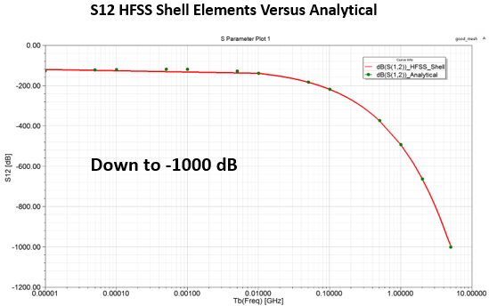
This example models a plane wave incidence on a finite thickness copper slab:

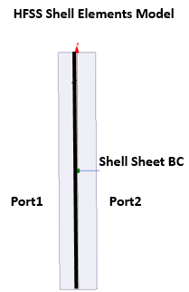
Simulations comparing HFSS Shell Elements to analytical show accuracy down to -1000 dB.

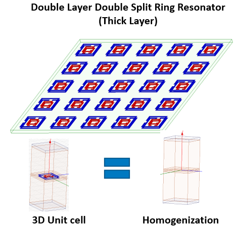
Simulation results compared.

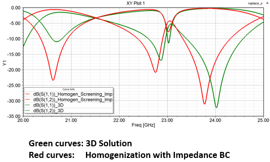
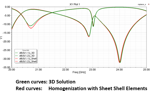
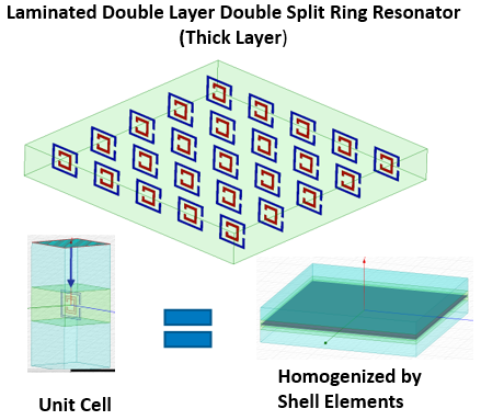
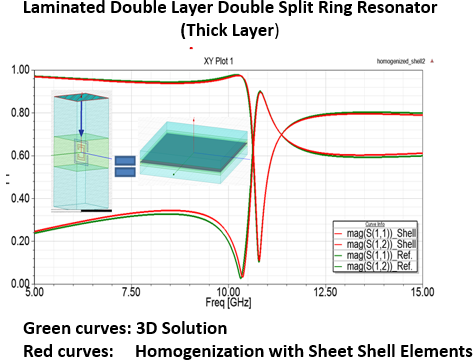
Simulation results compared.

Conclusions

• Shell elements are applicable both for conductive and dielectric layers.
• Broad band frequency sweep
• For dielectric layers, the accuracy deteriorates in relation to the how off normal the angle of incident is from the boundary. If the layered impedance boundary or shell element contains at least one high conductivity layer, then the accuracy maintains for a significant extent off normal.
• This dependence is much less when using layers with high conductivity.
• Numerical shell elements work well by using Unit Cell Data Link.
• Volumetric shell elements are accurate even with non-conformal mesh.

References

IEEE TRANSACTIONS ON MAGNETICS, VOL. 52, NO. 3, March 2016, "Modeling Periodic Layered Structures by Shell Elements Using the Finite-Element Method" by I. Bardi, G. Peng, and L. E. R. Petersson