Adding an SIwave-PSI Solution Setup

This section provides step-by-step instructions for configuring an SIwave-PSI solution setup within either the General or IC mode environments.

1. Open the SIwavePSISetup1 window. There are several ways to do this, depending on the current environment. For example:
   • From the Project Manager window, expand the Project Tree > [Active Design Folder]. Then right-click EMDesign1 or Analysis and select Add SIwave Solution Setup > Add SIwave-PSI Solution Setup.
   • From HFSS 3D Layout, select Solution Setup > select Add SIwave Solution Setup > Add SIwave-PSI Solution Setup.
   • From the Simulation tab, click SIwave-PSI.

2. From the Setup window, make selections from the General, Net Processing, Power/Ground Nets, Signal Nets, and Defaults tabs.

   

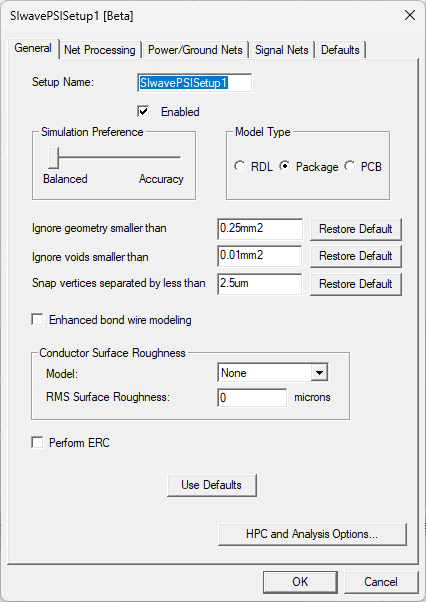
3. From the General tab, set the following:

   • Setup Name – type a name in the field or accept the default

   •  Enabled – check the box to activate or deactivate the setup

   •  Simulation Preference – use the slider to set the simulation to Balanced (i.e., use less memory) or Accuracy (i.e., use more memory)

   •  General Mode Only:

     • Model Type – select RDL, Package, or PCB.

       • PCB – for full board layout.

       • Package – for physical enclosure and interconnects.

       • RDL – for integrated circuit or interposer-level analysis.

     • Ignore geometry smaller than – enter a value and specify the unit. If applicable, you can Use Defaults.

     • Ignore voids smaller than – enter a value and specify the unit. If applicable, you can Use Defaults.

     • Snap vertices separated by less than – enter a value and specify the unit. If applicable, you can Use Defaults.

     • Enhanced bond wire modeling – check the box to activate. This can slow simulation.

   • Conductor Surface Roughness area – select a roughness model type from the drop-down menu (i.e., None, Exponential, or Hammerstad) and enter a variable in the RMS Surface Roughnessfield to specify the surface in microns.

   • General Mode Only: Perform ERC – check the box to determine whether to perform error checking while generating the solver input file.

   • HPC and Analysis Options – open a window allowing you to specify HPC options

4. Click the Net Processing tab.

   

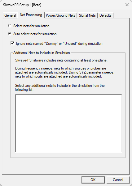
5. From the Net Processing tab, set the following:

   • Select Select nets for simulation (i.e., allows you to manually select nets to include in the simulation) or Auto select nets for simulation (i.e., allows HFSS 3D Layout to select nets to include in the simulation)
   • Ignore Nets Named "Dummy" or "Unused" during simulation – check the box to ignore dummy nets
   • Additional Nets to Include in Simulation – when Auto select nets for simulation is selected, select additional nets that must be included

6. Click the Power/Ground Nets tab.

   

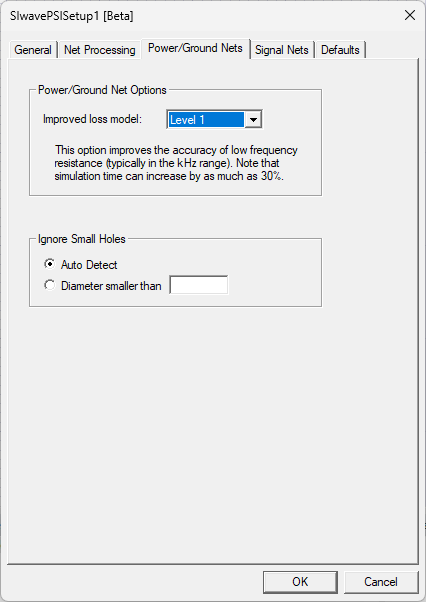
7. From the Power/Ground Nets tab, set the following:

   • Improved loss model – select an accuracy level from the drop-down menu (i.e., Level 1, Level 2, or Level 3)

     Warning:

     Simulation time increases at higher levels, by as much as 30%.

   • Ignore Small Holes – select Auto Detect (i.e., allow the software to detect and ignore small holes) or Diameter smaller than and enter a parameter in the field (i.e., specify a diameter and holes smaller than the diameter will be ignored)
8. Click the Signal Nets tab.

   

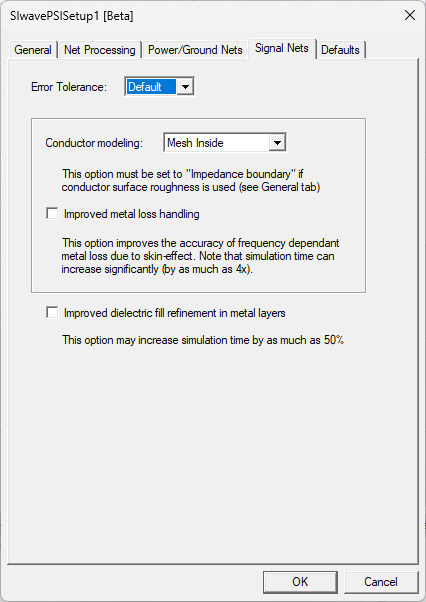
9. From the Signal Nets tab, set the following:

   • Error Tolerance – select a tolerance level from the drop-down menu (i.e., Default, 0.02, 0.04, 0.06, 0.08, 0.1, 0.2, 0.5, or 1.0)
   • Conductor Modeling – select Mesh Inside or Impedance Boundary from the drop-down menu
     Important:

     When using surface roughness, users must select Impedance Boundary from the Conductor Modeling drop-down menu.

   • General Mode Only: Improved Metal Loss Handling – check the box to activate.
     Warning:

     Enabling this option can significantly slow simulation time.

   • Improved Dielectric Fill Refinement in Metal Layers – check the box to activate or deactivate Improved Dielectric Fill Refinement
     Warning:

     Activating Improved Dielectric Fill Refinement in Metal Layers can significantly slow simulation time.

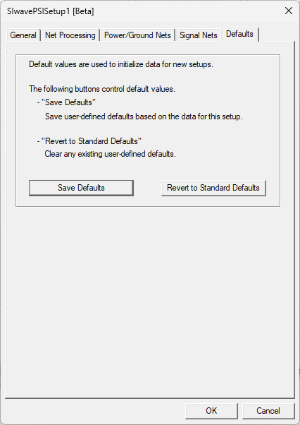
10. Click the Defaults tab.

    

11. From the Defaults tab, either Save Defaults or Revert to Standard Defaults.

12. Click OK to add the SIwave-PSI solution setup to the active design and simultaneously open the Edit Frequency Sweep window.

    

13. From the Edit Frequency Sweep window, click OK to accept the sweep with its default values or specify the following:

    Note:

    The available tabs and options change with the selected sweep type.

    • Sweep Name field – enter a name for the sweep.

    • Sweep Type drop-down menu – select Discrete or Interpolating:

      • Discrete – Generates field solutions at specific frequency points in a frequency range. Ideal when only a few frequency points are appropriate to accurately represent the results in a frequency range.

      • Interpolating – Estimates a solution for an entire frequency range. Ideal when the frequency range is wide and the frequency response is smooth. When Interpolating is selected, the Interpolation tab appears.

        Note:

        The information specified for an Interpolating sweep dictates the amount of information that can be viewed on a post-processing plot.

    • Enabled – check to enable the sweep.

      • Frequency Sweeps area – use Add Above, Add Below, and Delete to add or remove sweeps. Each row in the table represents a separate sweep and each column is either a selectable parameter or a value field. You can add multiple frequency sweeps to the same setup. Specify the Start and End frequency for each sweep, and make selections from the additional options specific to the Distribution type.

        Note:

        IC Mode Only: If the user enters 0MHz in the Start value field, the Ansys Electronics Desktop (AEDT)^TM electronics systems design platform can use a DCIR solver within the SIwave-PSI simulation to calculate DC point.

        

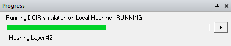
        To activate this beta feature, navigate to the Beta Options window as described in Activating the SIwave-PSI Solution Beta Feature steps 1-2, then check the box adjacent to DCIR solver support for SIwave-PSI in IC Mode.

        • Distribution – select from the following:

          • Linear Step – A linear range of frequency points for which users specify a constant step size. The simulation will solve the frequency point at each step in the specified frequency range, including the start and stop frequencies (e.g. , specifying 10 for the Start frequency, 20 for the Stop frequency, and 2.5 for the Step Size instructs the simulation to compute a solution for frequencies of 10, 12.5, 15, 17.5, and 20).

          • Single Point – Individual frequency points. Insert specific frequency points to solve in the frequency range after uniform frequency points. For Discrete sweep types only.

          • Single Point Sweep – Adds a set of 10 Single Point Sweeps, defaulting from 1 GHz to 10 GHz in increments.

          • Linear Count – A linear range of frequency points for which users specify the number (count) of points within the frequency range. The simulation divides the frequency range into the count specified and solve each frequency point in the count.

          • Log Scale – A range of points for which users specify Start, End, and the number of Samples.The simulation assigns the sampled points using intervals based on a logarithmic scale.

• Click Preview to view a preview of the sweep, as currently defined.

  

• From the Sweep Options area, check boxes to activate any/all of the following options:

  Note:

  Sweep Options are only available if the Sweep Type is Interpolating.

  • Fast Sweep check box – check to improve runtime by requiring fewer samples to simulate. Uses more memory.

  • Adaptive Sampling check box – check to determine the number of sample frequency points from the response over the frequency band, adding more points around rapidly changing responses (e.g., resonance peaks). Checking the Adaptive Sampling box activates the Enforce causality and use enhanced AC/DC merge box.

    • Enforce causality and use enhanced AC/DC merge check box – check to enforce causality and generate S-parameters at the DC point. By combining the DC results with the frequency-swept AC results, accuracy is improved over the entire simulation bandwidth.

14. Click OK to close the Edit Frequency Sweep window and add any sweeps.

15. From the Edit Frequency Sweep window, click OK to accept the sweep with its default values or change the default values. Refer to Adding a Frequency Sweep for more information.

16. IC Mode Only: If applicable, apply a technology file to the design.

    Note:

    Encrypted technologies are only supported by HFSS, Q3D, and RaptorX simulations.

17. Run the analysis to solve the setup. Refer to Running Simulations.

18. To add a PI type:
    1. From the Layout Editor, select the port.
    2. From the Properties window, select the EM Design tab. Then click the SIwave-PI Type value field and select from the following:
       • Default (the initial condition of a new port)
       • Coaxial Open
       • Coaxial Shorted
       • Gap
       • Lumped

The procedure is complete.

Activating the SIwave-PSI Solution Beta Feature

Follow these steps to enable the SIwave-PSI Solution Setup beta feature.

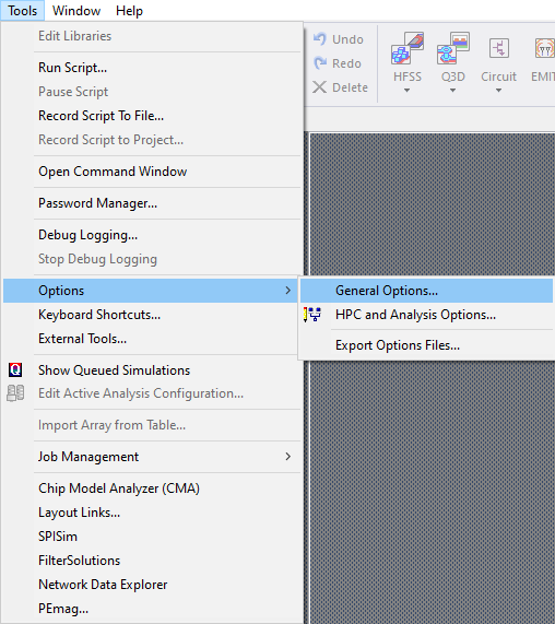
1. From the Tools menu, select Options > General Options to open the Options window.

   

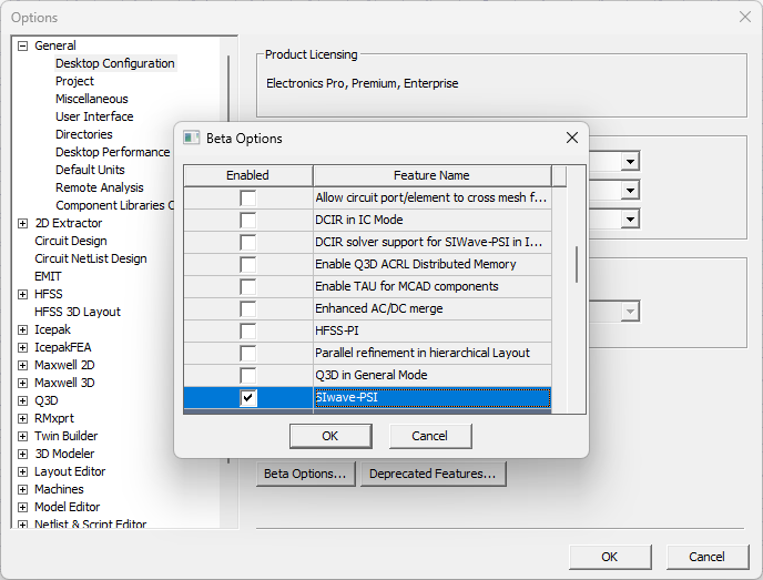
2. Expand General > Desktop Configuration and click Beta Options to open the Beta Options window.

3. Scroll down and check the SIwave-PSI box.

4. Click OK to close the Beta Options window.

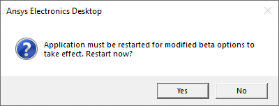
5. Click OK to close the Options window and open a prompt to restart the software. Users may be asked to save their work.

   

6. Click Yes to restart immediately.

7. After restarting the software, the SIwave-PSI solution setup is available from the locations described in the previous section.

The procedure is complete.