Exporting Macro Model

Network Data Explorer lets you export macro model data. To export data, click the Broadband icon on the NDE ribbon.

The Broadband Export Options dialog box appears.

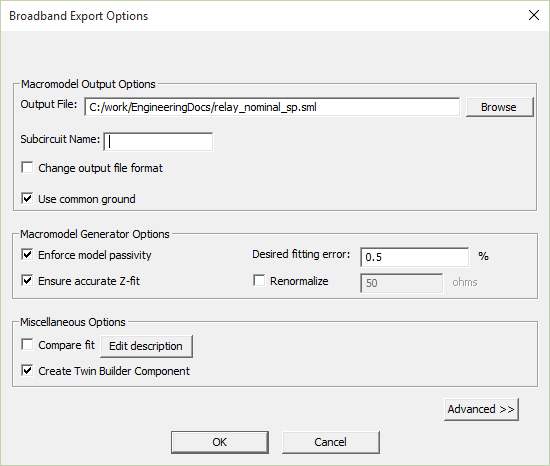
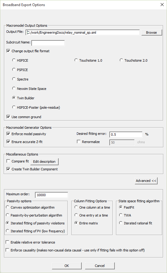
Click Advanced >> to view all options.

Macromodel Output Options

• Output File – Choose the name and location of the file.
• Subcircuit Name – Name the subcircuit.

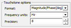
• Change Output File Format – Select this box to choose an output format from the list.

  When you select Touchstone 1.0 or Touchstone 2.0 as the format, the following Touchstone options appear:

  

• Use common ground – Select this box to use common ground. When this option is on, ports are referenced to ideal ground (node 0). When this option is off, extra ports generate to provide reference levels. Common grounding is best when the pins are physically near to each other and ideal ground is suitable. For distant connections and circuits with non-ideal reference levels such as differential pairs, common grounding is not used.
Note:
• R and L values may be quite sensitive to the values of the S-parameters. This is an issue if the actual impedance value is much greater than, or much less than, the reference impedance of the S-parameters.
• Since resistances of power cables is typically in the milliohms range at DC, using a reference impedance = 50 ohms is 5000 times higher. This causes any fitting errors in the state space model to get multiplied by 5000 times when the R and L values are computed.
• As a general rule, for high power applications a reference impedance of 1 ohm is probably a better choice than 50 ohms.

Macromodel Generator Options include:

• Enforce Model Passivity – Select this box to enforce passivity. A uniform renormalization of 50 ohms is performed on the solution data for passivity checking.
• Ensure Accurate Z-fit – Select this box when state-space fitting of Y-parameters or Z-parameters does not produce an accurate fit.
• Desired Fitting Error – Select the value at which rational fitting fails (if the fitting error exceeds this value).
• Renormalize – Select this box to renormalize using the impedance specified in the adjacent text box. 50 ohms is the default value, but you can enter a different value.
Note:

R and L values may be quite sensitive to the values of the S-parameters. This is an issue if the actual impedance value is much greater than (>>) or much less than (<<) the reference impedance of the S-parameters.

Since resistances of power cables is typically in the milliohms range at DC, using a reference impedance = 50 ohms is 5000 times higher. This causes any fitting errors in the state space model to get multiplied by 5000 times when the R and L values are computed.

As a general rule, for high power applications a reference impedance of 1 ohm is probably a better choice than 50 ohms.

Miscellaneous Options

• Compare Fit – When this box is selected, the original and derived solution will be available for comparison. Click Edit Description to open the Derived Solution Description dialog box and add a text description to better identify the export.

  

• Create Twin Builder Component – Creates a Twin Builder component. This option is available only for Twin Builder designs.

Advanced Options

The following advanced options are available:

• Maximum order – Number of poles. The Broadband models are built from a rational-function approximation to the data. The fidelity of this approximation can be controlled by setting the Desired fitting error and the Maximum order (number of poles).
• Passivity Options – If you enabled Enforce Model Passivity, this area lets you select the passivity enforcement method.
• Convex optimization algorithm – Guarantees a passive state-space realization, but is very slow and memory-intensive.
• Passivity-by-perturbation algorithm – Designed for systems with a large number of ports.
• Iterated fitting of passivity violations (IFPV) (default) – Less accurate than other algorithms but quickly estimates a fit with low memory usage.
• Iterated fitting of PV (low frequency) – Similar to IFPV while improving the fit to “Z” at DC and low frequencies.
• Column Fitting Options
• One column at a time – The set of poles is shared across all entries of a single column.
• One entry at a time – Each entry is fitted using a separate set of poles.

• Entire Matrix – The set of poles is shared across all entries of the matrix being fitted.

  Note:

  • Typically, using the same set for all entries is adequate, and yields the most compact models. However, if all the entries of the matrix have completely unrelated transfer functions, it may be better to fit them using separate pole sets.

  • The options One column at a time and One entry at a time do not work when either Ensure accurate Z-fit or FastFit is used.

• State space fitting algorithm – Select either FastFit, TWA, or Iterated rational function.

  • FastFit – FastFit is the Ansys-proprietary default method for state-space fitting. ndExplorer uses FastFit for calculating the state-space matrices from the network data. The FastFit algorithm for state-space fitting is an alternative to the Tsuk-White algorithm (TWA) and Iterated Rational Fitting (IRF) methods. FastFit is generally as accurate as TWA, but is significantly faster than both TWA and IRF. It also aims to fit the lower frequencies with higher fidelity.
  • TWA (Tsuk-White Algorithm) – An Ansys-proprietary method for fitting a state space model to extracted s-parameter data. It uses techniques based on Singular Value Decomposition (SVD) to quickly determine required number of poles for fitting a model.
  • Iterated rational function – This fitting approach takes a matrix of S-parameter data and, for each matrix entry, tries a succession of different pole-zero approximations (increasing the number of poles used at each iteration) until it can find an acceptable fit to the data. For broad frequency sweeps and large numbers of excitations, this process can be time consuming because of all the iterations and is not guaranteed to produce a good fit to the data. It is retained as a fallback if the TWA algorithm fails.

• Enable relative error tolerance – Enable relative error tolerance, which works best with the TWA algorithm.

  Note:

  Although the Enable relative error tolerance option works best with the TWA fitting algorithm, is not recommended for use with the Iterated rational function algorithm, and is disabled when FastFit or Ensure accurate Z-fit is used.

• Enforce Causality (makes non-causal data causal-use only if fitting fails with this option off) – Select this box to enforce causality when needed for fitting to succeed. Measurement noise or numerical simulation errors can result in data that cannot be approximated accurately with a moderate number of poles. In particular, the data may resemble the response of a non-causal system, and since the Broadband model is causal by construction, it becomes impossible to achieve a good fit. In such cases, you may use the Enforce Causality option to approximate the data as that of a causal system prior to fitting. However, doing so may introduce significant fitting errors with respect to the original data. This option should be used only when the fitting fails without it.

Click OK to begin the export. The Message Manager pane details the export process.

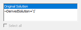
Comparing Original S-Parameters with Exported S-Parameters

~DerivedSolution='1' is the exported solution. If you selected the Compare fit check box during export, the data selection pane updates to list both the original and derived solution.