
Two-Way Coupling
This feature builds on the ability of Mechanical – Thermal solutions to import EM losses from one or more source designs. The two-way coupling capabilities in Ansys Electronics Desktop (AEDT) allow the temperature results from a Mechanical – Thermal solution to be fed back to an EM loss source design, in which another solution iteration is then performed. Temperature-dependent materials in the source design are affected by the fed-back temperature distribution, thus altering the results of the source solution (and likely changing the EM loss results). A solution controller coordinates the iterative process, next running another iteration of the thermal solution, feeding back the updated temperature distribution to the source design, and so on. The iterative process continues until the user-specified number of coupling iterations has been completed.
For a video presentation of the two-way coupling workflow, see the Overview Video page.
Two-way coupling is supported between Mechanical design thermal solutions and any of the design types that can be used as a source of EM loss data. Specifically, the supported design types are as follows:
- HFSS: From Modal, Terminal, or Eigenmode solutions – import surface losses from non-solve-inside conducting objects and volume losses from solve-inside lossy objects
- Maxwell 3D: Surface losses from Impedance boundaries, and volume losses from solve-inside conducting objects.
- Q3D: Surfaces losses from conducting objects for the AC field type, and volume losses from lossy objects for the DC field type
- Lossy objects are those with material definitions that include a Dielectric Loss Tangent greater than zero.
- For source designs with transient solutions, losses for time steps that are defined as a function (for example, a function of a time) cannot be mapped to a Mechanical thermal solution.
Two-Way Coupling Requirements
Beyond the requirements for importing EM loss results, the following additional requirement must be satisfied in order to perform two-way coupling:
- For designs acting as EM loss sources:
- You must specify a temperature-dependent material for one or more objects.
- You must select both the Include Temperature Dependence and Enable Feedback options in the Temperature of Objects dialog box.
- For the Mechanical – Thermal design:
- For the coupled EM Loss excitations, you must select both the Simulate source design as needed and Preserve source design solution options in the Setup Link dialog box.
- You must create a 2-Way Coupling solution setup (which is the controller for the two-way iterative solution process).
- Additional restrictions:
- The Mechanical – Thermal design is restricted to a single solution setup.
- Coupled upstream simulations (EM loss source designs) must be driven via the controller in Mechanical. Any simulation you directly initiate at the upstream design will likely cause the next coupled Mechanical simulation to restart from iteration 1.
- Do not use post processing variables in the upstream designs (for example, post processing variables in the HFSS Edit Sources dialog box). When post processing variables are used in upstream designs, the coupled solution can become out of sync with its nominal variation.
- Do not edit the upstream design during a coupled simulation.
- An HFSS, Maxwell 3D and Q3D design can only couple with AEDT Mechanical via the AEDT controller. These source designs can be coupled with Ansys Workbench–Mechanical when they are not coupled with AEDT Mechanical. A Maxwell 3D design can be coupled with AEDT Mechanical when it is not already coupled via Command Line System Coupling or Workbench.
- Q3D solution setups with more than one problem type enabled are not supported.
- Frequency sweeps in Q3D solutions are not supported. Imported EM losses are only available at the Solution Frequency specified under the General tab of the Solve Setup dialog box.
Two-Way Coupling Workflow
Within the following procedure, the terms upstream and downstream are used to identify the designs or solutions. Upstream refers to the design that is the source of the EM loss results. Downstream refers to the Mechanical – Thermal design into which the EM loss data is imported and resultant temperatures are computed.
- Create two designs using identical geometry and object names. One will be a Mechanical – Thermal design and the other must be a design type supported as an EM loss source (HFSS, Maxwell 3D, or Q3D).
- In the upstream design, assign temperature-dependent material properties to one or more parts.
- Search the applicable product's help for "specifying thermal modifiers". (The quotation marks limit search results to instances of the full phrase.)
- For information concerning supported operators and constants that you might want to use in a thermal modifier expression, search applicable products for
- In the Project Manager, right-click the upstream design and choose Set Object Temperature from the shortcut menu.
- In the Temperature of Objects dialog box that appears, select the following two options:
- Include Temperature Dependence
- Enable Feedback
- In the Mechanical – Thermal design, assign an EM Loss excitation to one or more objects, setting up a link to the source design and ensuring that the imported loss is correctly assigned as a Surface or Volume loss.
- Ensure that required boundaries, excitations, and solution setups are fully defined for both the upstream and downstream designs.
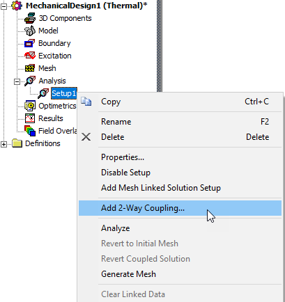
- In the Mechanical design, right-click the analysis setup in the Project Manager and choose Add 2-way Coupling:
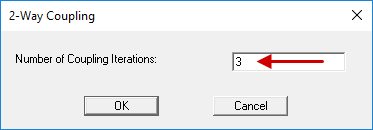
- In the 2-Way Coupling dialog box that appears, specify the desired Number of Coupling Iterations and click OK. This value must be a positive integer.
- When all coupled iterations have been completed, right-click the mechanical solution setup, under Analysis in the Project Manager, and choose Profile.
- Compare the reported Total Loss on Source Object values for the last two iterations:
- Depending on the comparative Total Loss on Source Object results, choose one of the following three actions:
- If the changes in the total loss results are insignificant between the last two completed iterations, consider the coupled solution converged. The two-way coupled analysis is finished. Continue to step 12.
- If the total loss results significantly differ between the last two completed iterations, increase the specified Number of Coupling Iterations and resume the two-way coupled analysis as follows:
- In the downstream design, under Analysis > mechanical solution setup in the Project manager, double-click 2-Way Coupling.
- Increase the value in the Number of Coupling Iterations text box, and click OK.
- Right-click the mechanical solution setup in the Project Manager and choose Analyze.
- When you restart the solution, it proceeds immediately to the next iteration using the field results from the last one completed.
- The Profile retains the history of all previously run and new iterations.
- Go to step 9 and continue again from there.
- If the solution is diverging or the results are oscillating significantly, recheck boundaries, excitations, material properties, and mesh quality. Divergent or oscillatory solutions are more likely when one or more materials in the source design have a highly nonlinear conductivity or loss tangent. Tightening the convergence tolerance and increasing the maximum number of passes in the source solution setup may be helpful.
- Complete the post processing phase (create desired reports and field overlays).
Vacuum or air regions needed for field calculations in the source design may or may not be applicable to your thermal analysis. All thermal design objects must have non-zero thermal conductivity. When you import or copy a vacuum object into a Mechanical – Thermal design, if a nonzero thermal conductivity has not previously been specified in the vacuum material's properties, the material air is automatically reassigned to the object. Otherwise, if air or vacuum regions are not relevant to the thermal solution, you can delete them from the Mechanical design or set them as non-model parts. However, note that you will not be able to import the source design's mesh after removing or deactivating any objects within the Mechanical design (the geometry will no longer be identical to the source design).
For information concerning the definition of temperature-dependent material properties, consult the following references:
Alternatively, you can click the product menu (HFSS, Maxwell 3D, or Q3D and choose Set Object Temperature.
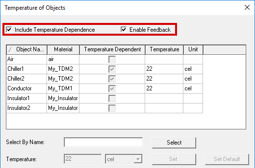
The check boxes in the Temperature Dependent column indicate which objects have temperature-dependent material properties assigned to them.
The Solutions dialog box appears with the Profile tab selected.
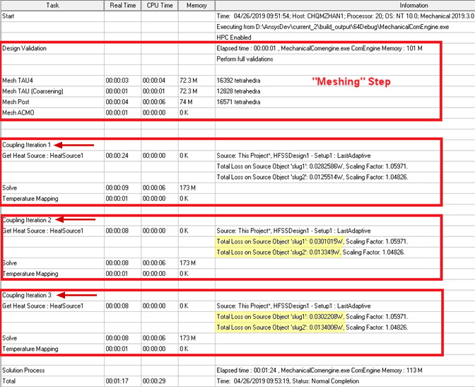
You can judge whether you've run a sufficient number of coupling iterations by comparing the Total EM Loss magnitudes between the last two iterations (highlighted in the preceding Profile image). Convergence occurs when the EM losses and resultant temperatures stabilize (that is, when the variation in these results between adjacent iterations becomes insignificant). However, in certain cases a solution may not stabilize, and you may experience an oscillatory or divergent (runaway) solution. If the total EM losses oscillate (that is, continue to repeat an increase/decrease cycle), the solution still may be acceptable if the magnitude of the change is relatively small.
After revising the source design, return to the target design, clear the linked data, and rerun the coupled analysis.
Solution Invalidation
Previously solved results are invalidated when you delete the 2-Way Coupling setup or when you right-click the solution setup in the Project Manager and choose Revert Coupled Solution from the shortcut menu.
The controller automatically detects “out of sequence" simulations and restarts the coupled analysis. The following message is posted in the Message Manager window when a coupled simulation needs to be restarted:

Examples of out of sequence simulation situations include:
- Source design edits have been made that invalidate the source design solution.
- Target design edits have been made that invalidate the controller data, including edits that invalidate the imported EM Loss data. Examples include changes in mesh and geometry.