Assigning a Voltage Excitation
To set a voltage excitation for the 3D AC Magnetic A-Phi Solver:
- Select the section of the geometry on which you want to apply the excitation.
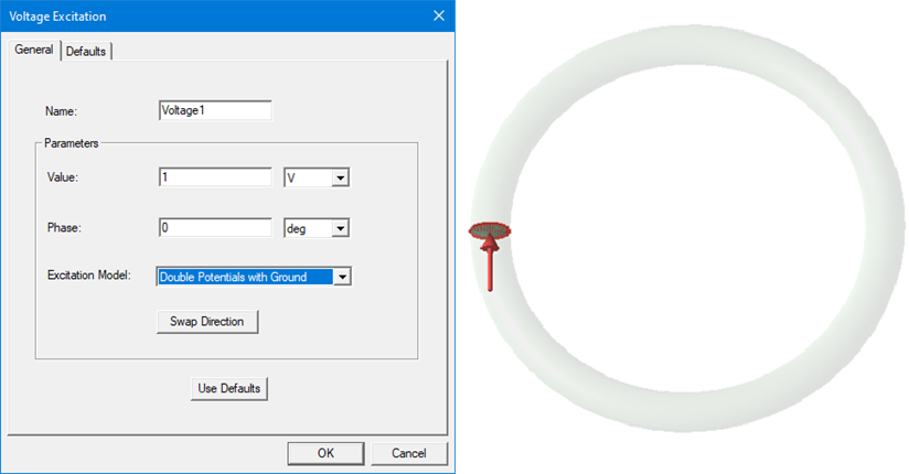
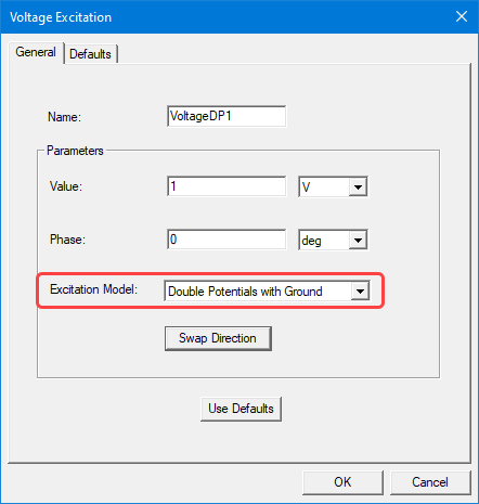
- Click Maxwell 3D > Excitations > Assign > Voltage. The Voltage Excitation window appears.
- Enter a name for the excitation in the Name field, or accept the default.
-
In the Parameters section:
- Enter the electric potential in the Value field, and select the unit from the drop-down menu. You can enter a numerical value.
- Enter a value in the Phase field, and select a unit from the drop-down menu.
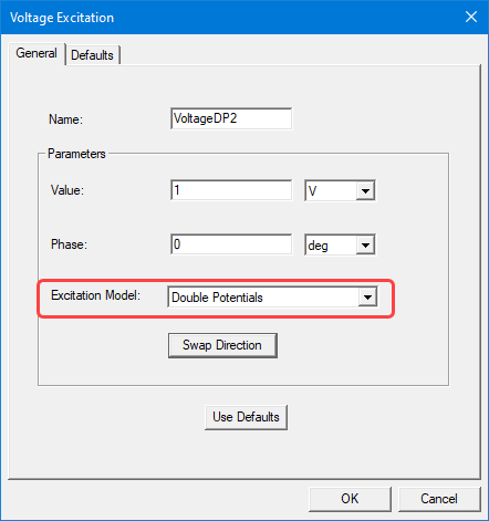
- Choose the Excitation model. Refer to the next section for details on the options.
- Optionally, to change the direction of the voltage flow, click Swap Direction.
- Optionally, click Use Defaults to revert to the default values in the window.
- Click OK to assign the excitation to the selected object.
Excitation Models
Voltage excitation supports three different excitation models: Single Potential, Double Potentials, and Double Potentials with Ground.
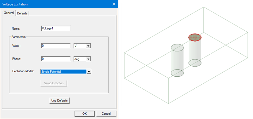
Single Potential
The solver treats the terminal as an equipotential terminal. Only one scalar electric potential DOF (Degree of Freedom) is assigned to the surface, and the value of the DOF is set to the value that the user inputs.
Double Potentials
The solver treats the terminal as a voltage (potential drop) terminal. At the terminal face, two scalar electric potential DOFs are defined, and the DOFs are unknown. The difference between those potentials equals the voltage value that the user specified. If the voltage value is a positive quantity, the higher potential is in the specified direction.
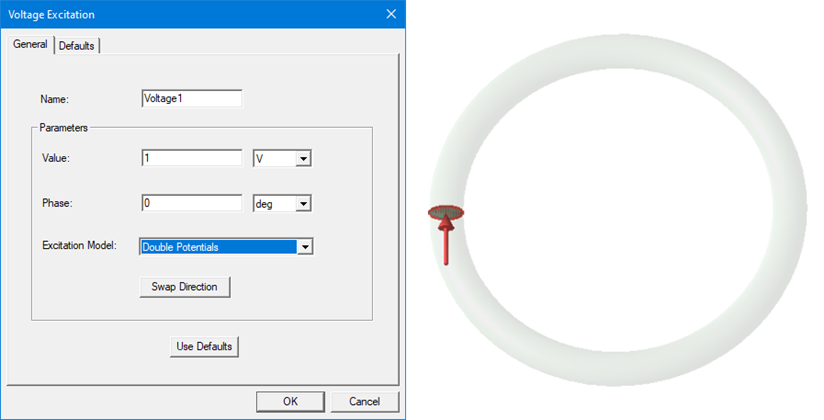
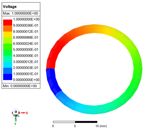
The voltage profile for Double Potentials is shown below:
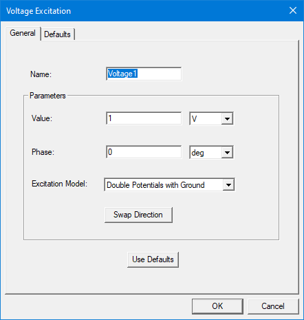
Double Potentials with Ground
The solver treats the terminal as a voltage (potential drop) terminal. At the terminal face, two scalar electric potential DOFs are defined, and both DOFs are known. The difference between those potentials equals the voltage value that the user specified. If the voltage value is a positive quantity, the DOF in the specified direction is set to the specified voltage value, and the DOF in the opposite direction is set to 0.
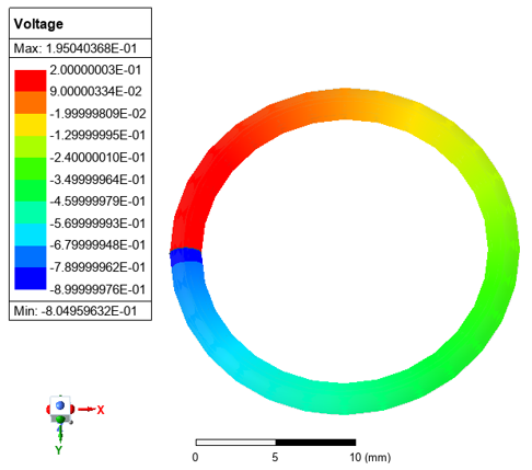
The voltage profile for Double Potentials with Ground is shown below:
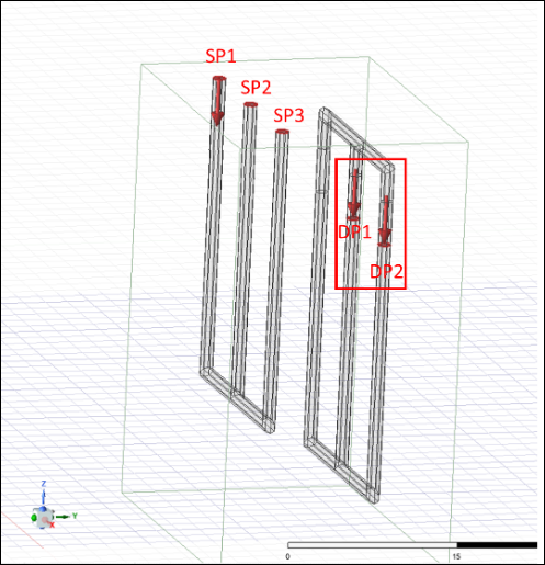
Closed Loop Excitations
To simulate closed loop excitations, the Excitation Model should be Double Potentials or Double Potentials with Ground:
The figure that follows shows an example of closed loop excitation (DP1 and DP2) assignments. Multiple terminals assigned on one conduction path are also supported; see single potential excitation (SP1, SP2, SP3) assignments in the figure that follows.