
Incident Plane Wave
A plane wave is a wave that propagates along a fixed direction where the electric and magnetic fields are in the transverse plane and perpendicular to each other.
A plane wave is defined by the following equation:


The term k represents the wave number of the global background material for regular/propagating plane waves.
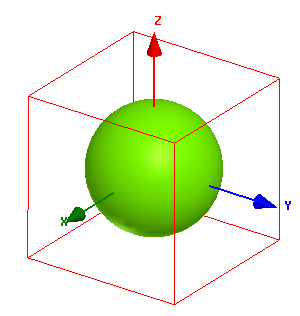
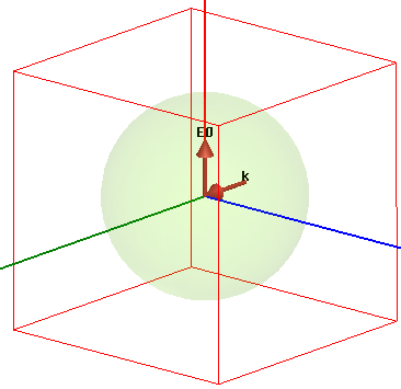
An HFSS model of a dielectric sphere is shown to illustrate the incident plane wave setup.
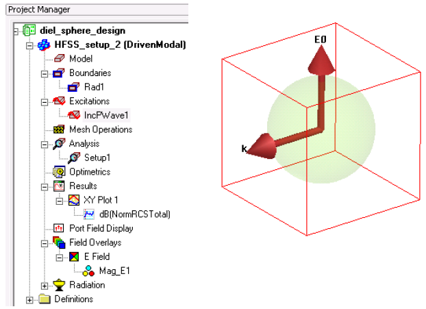
After a plane wave is defined, the propagation direction and the electric field direction can be visualized as shown in the following figure.
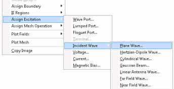
To define a plane wave, right-click anywhere in the Modeler and select Assign Excitation> Incident Wave> Plane Wave.
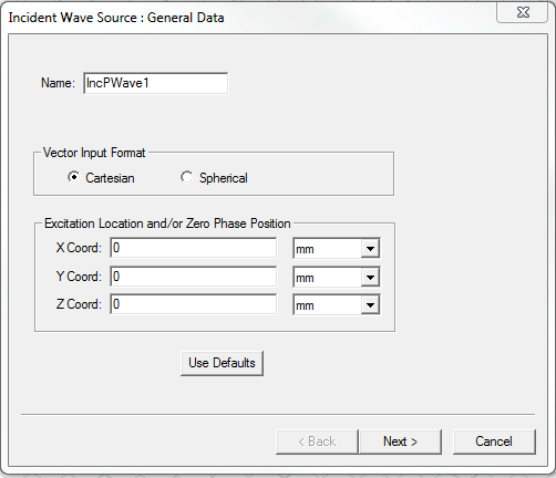
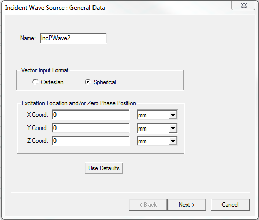
The Incident Wave Source: General Data dialog box appears. You can select either Cartesian or Spherical for the Vector Input Format.
Cartesian Vector Setup
Enter the Cartesian co-ordinates on the Incident Wave Source: General Data dialog box to set the zero phase location for propagating wave and click Next.
For evanescent waves, Cartesian co-ordinates are defined for the Excitation location.
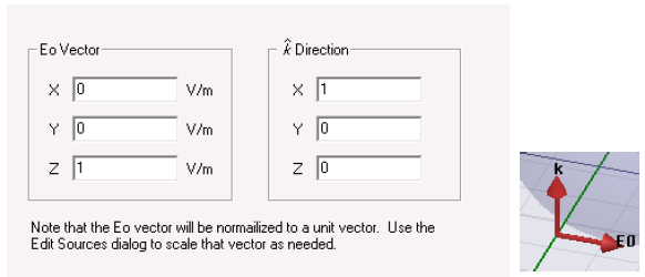
The following figure shows the Cartesian Vector Setup panel. Define the direction of Eo. Regardless of the magnitude of the field vector Eo, HFSS normalizes it to 1. However, the magnitude of Eo can be scaled to the desired value on the Edit post process sources panel.
Also, define the direction of the unit vector of propagation,
 . It is your
responsibility to ensure that the direction of propagation,
. It is your
responsibility to ensure that the direction of propagation,  of the plane wave
is perpendicular to E0.L
of the plane wave
is perpendicular to E0.L
Click Next to specify the the type of plane wave on the Plane Wave Optionspanel.
Recall the equation that describes a plane wave:


where k is the wave number of the global background material for regular/propagating plane waves. In most cases, the values defined for Eo and k are meant for regular/propagating plane waves. For evanescent waves, since k = b + ja it overrides the magnitude of the complex propagation constant.
In HFSS, evanescent waves do not depend upon the global background material. However, the post-processed near or far fields depend upon the global background material. For more information see the section Global Material Environment.
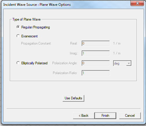
If you select the type of plane wave as Elliptically Polarized, specify the ratio of the large axis to the small axis of the ellipse and the phase angle of the large axis. For more information, see the section Elliptically Polarized Plane Wave.
Spherical Vector Input Format
This section demonstrates the same incident plane wave by defining the vector input format for a Spherical setup.
- On the Incident
Wave Source: General Data dialog box, select the option Spherical.
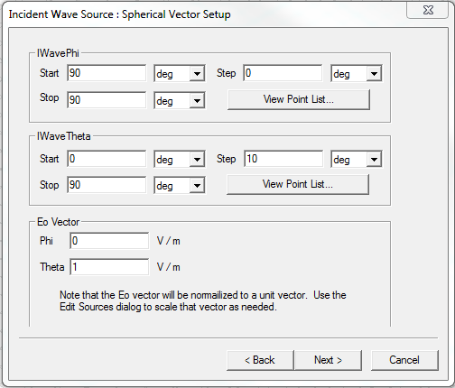
- Click Next and edit the IWavePhi,
IWaveTheta, and Eo
Vector fields as shown in the following figure.
This setup provides an alternate way of defining plane waves using spherical vector format. The orthogonality of
 and Eo is
automatically satisfied since
and Eo is
automatically satisfied since  is in the
  direction. Regardless of the magnitude of Eo,
HFSS normalizes it to 1. However, the magnitude of Eo can be scaled
to the desired value on the Edit post process sources panel.
direction. Regardless of the magnitude of Eo,
HFSS normalizes it to 1. However, the magnitude of Eo can be scaled
to the desired value on the Edit post process sources panel.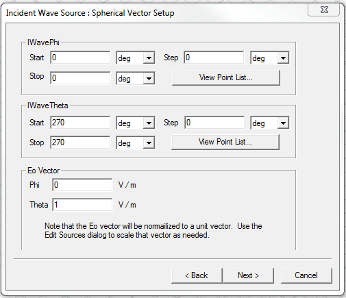 Note:
Note:If you enter values in the Step fields and click the View Point List button, you can see all the phi or theta values.
For a spherical incident wave you can specify an expression to define an angle in the start field only. If use an expression, the dialog disallows any stop/step values. In other words, we allow only a single angle if you choose to parametrize the start angle.
You can visualize the propagation direction and the electric field direction for a plane wave defined for spherical vector setup as shown in the following figure.
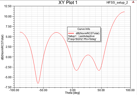
The normalized bistatic RCS plot for theta scan at phi = 0 plane is shown below.
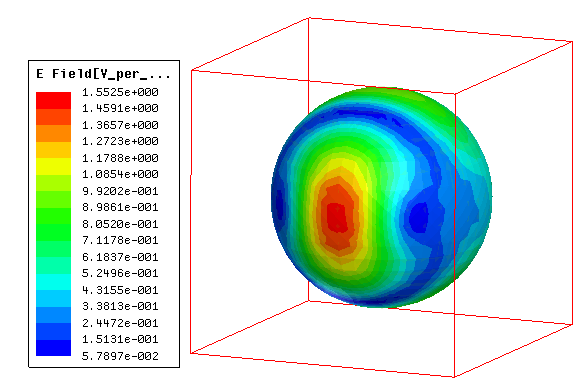
The following figure shows the scattered E-field plot on the surface of a dielectric sphere (radius = 30mm, relative permittivity = 10, and solution frequency = 5 GHz.)
The Spherical vector input format provides a convenient way of specifying multiple incident angles.
Defining Multiple Plane Waves
This section describes how to define multiple plane waves using Spherical Vector Setup.
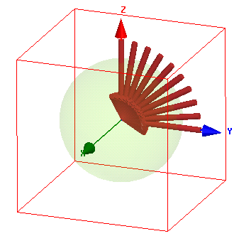
The following figure shows the Spherical Vector Setup panel. An incident wave sweep is defined in the phi = 90 degrees plane for theta, with step size of 10 degrees.
This setup defines eleven incident plane waves as source as shown in the following figure.
The following figure shows the scattered E-field plot on the surface of the dielectric sphere (radius = 30mm, relative permittivity = 10, and solution frequency = 5 GHz) at incident angle of theta = 40 degrees.
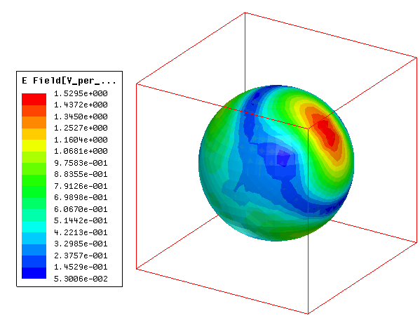
This E-field plot is defined for IWaveTheta = 50 deg and IWavePhi = 0 deg.
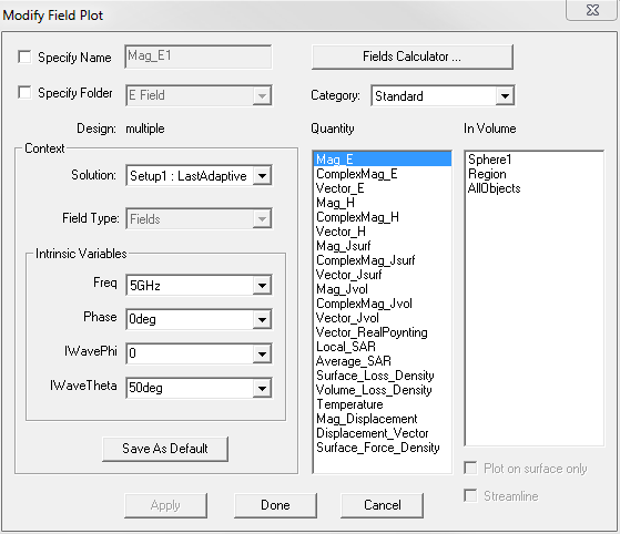
Although the incident field sweep defines multiple plane waves, only one scale factor is applied on all the plane waves. This scale factor can be edited on the Edit post process sources panel.
Both the overlay field panel and the Reporter provides you options to select the desired incident plane wave.