
HFSS RF Discharge
HFSS RF Discharge targets applications related to aerospace and satellite communications where electrical breakdown in gases is a concern. A small number of free electrons naturally exist in gases due to photoionization and irradiation. When the electrons are accelerated by RF/microwave waves, they gain enough kinetic energy to ionize neutral gas atoms or molecules. The ionization is easier to happen at high altitudes or a space environment due to low gas pressures and abundant cosmic rays. If the number of electrons grows exponentially due to cumulative ionization, it can eventually trigger a discharge to damage RF/microwave circuits and sources. At high frequencies, the discharge mainly depends on the electron transport properties of the gases rather than the electron emission properties of the electrodes. This tool solves for the condition which leads to the onset of gas discharge not completely bridging material walls.
An RF discharge analysis is useful for predicting electrical breakdown in the following applications:
- TT&C (Telemetry, Tracking, and Command) subsystem switched on during satellite launching
- Uplink transmission to communication satellites
- Outgassing during the lifetime of satellites or space probes
- Re-entry vehicles and interplanetary missions
- Airborne radars and communication systems
It requires the time-harmonic fields being solved for a driven-terminal or driven-modal projects. Therefore, the RF discharge setup and associated DC magnetic bias (possibly nonuniform through Maxwell link) should be added to aforementioned types of HFSS projects. You can also perform an RF Discharge simulation on an Eigenmode solution. Other solution types, such as Transient, Characteristic Mode, and SBR+, do not support the RF discharge analysis. By option, you can save and plot electron density data.
Prerequisites
The Solution type must be Driven Terminal or Driven Modal or Eigenmode.
Save Fields for a Driven Terminal or Driven-Terminal Project
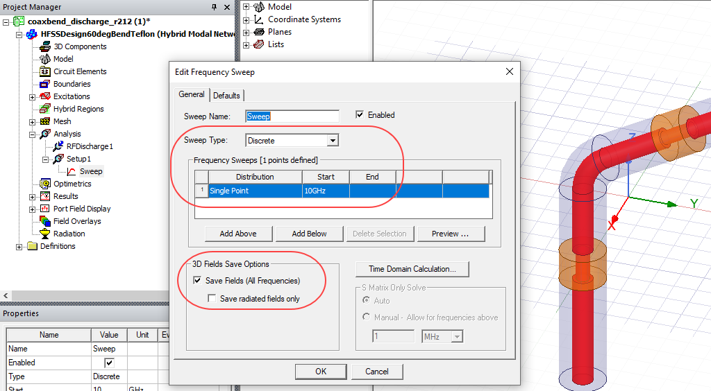
An RF discharge simulation requires time-harmonic fields as excitations. You must edit the frequency sweep of a driven-modal or driven-terminal project to save fields. However, storing fields takes time and disk space, especially when the size of the project and the number of frequency points are large. In addition, the RF discharge solver will solve one Paschen curve for each frequency. To reduce the simulation time and avoid clogging the RF discharge plot, should create a frequency sweep with few frequency points for linking with an RF discharge analysis. A frequency sweep for interpolating sweep of S-parameters over hundreds of frequency points is not suitable for linking with an RF discharge analysis.
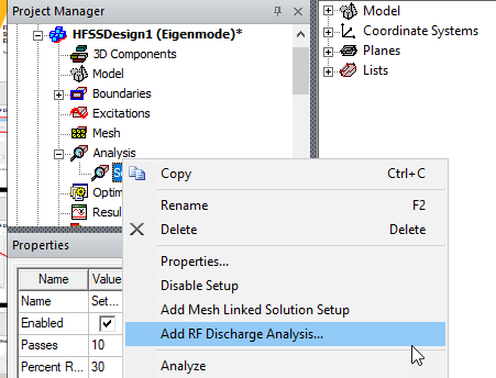
Add an RF Discharge Analysis to a Driven Solution
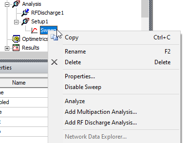
An RF discharge analysis can be created only when there is a frequency sweep with 3D Fields Save Options checked. Otherwise, the featured is grayed out. Right click the frequency sweep to Add RF Discharge Analysis.
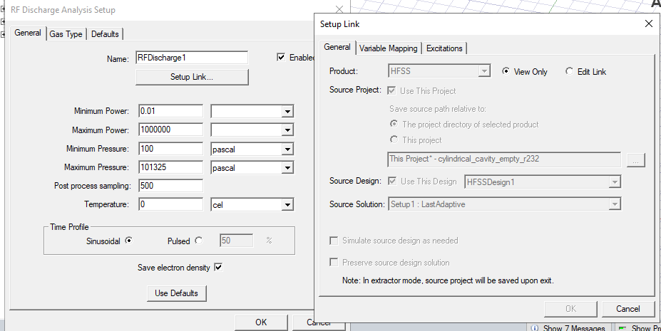
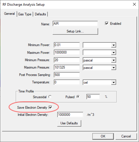
The RF Discharge Analysis Setup dialog lets you specify General parameters for Maximum and Minimum Power and pressure, as well as sampling and temperature values.
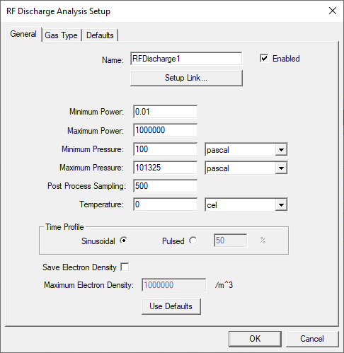
By default, the pressure ranges from 0.1 to 101.325 kPa. You set appropriate power and pressure bounds according to the operating range of your designs.
Select the Source and Port Excitations
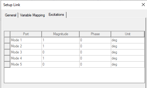
A driven design must contain at least one active frequency sweep with at least one active port for you to set up the source link. When the solution type is Modal Network or Terminal Network, the total field used in discharge simulation is a linear combination of field patterns of individual ports weighted by the complex multipliers (phasors) listed in the table. You set the input power of each active port on the Excitations tab of the Setup Link dialog to one Watt.
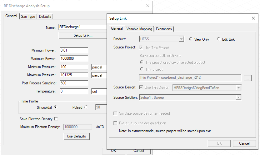
The total field used in discharge simulation is a linear combination of field patterns of individual ports weighted by the complex multipliers (phasors) listed in the table. You set the input power of each active port on the Excitations tab of the Setup Link dialog to one Watt.
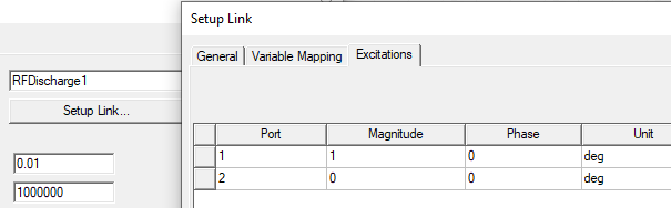
OK the Setup Link dialog box.
Gas Type for RF Discharge Analysis
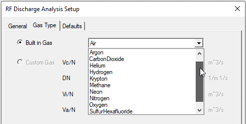
Click the Gas Type tab to select either Built-in or Custom gases. There are 12 built-in gases in the default gas library: Air, Argon, Carbon Dioxide, Helium, Hydrogen, Krypton, Methane, Neon, Nitrogen, Oxygen, Sulfur Hexafloride, and Xenon. Use the arrows to scroll through the drop-down list. Non-conductive materials in the simulation domain with relative permittivities no more than 1.02 and relative permeabilities in between 0.99999 and 1.00001 will be replaced by the gas selected from the list. For example, air and vacuum in the HFSS material library will be replaced according to the above rule.
A Custom Gas can be specified by four datasets of the electron collision frequency (Vc/N in m3s-1), the diffusion coefficient (DN in m-1s-1), the ionization rate (Vi/N in m3s-1), and the attachment rate (Va/N in m3s-1) as functions of the reduced electric field E/N (Td). If the project or the design does not have any dataset defined, the Custom Gas parameters will be grayed out on the Gas Type tab of the dialog.
Click OK to complete the setup.
Please note that the gas parameters of built-in gases are based on measured data with E/N between 0.1 and 5000 Td. The limitation may cause simulation results to deviate from ideal Paschen curves especially at low pressure.
Add an RF Discharge Analysis to an Eigenmode Solution
You can add an RF Discharge analysis to Eigenmode solution.
Use the Add RF Discharge Analysis... command to set parameters in the and Setup Link...
When the solution type is Eigenmode, the fields used in discharge simulation are individual field patterns of each mode weighted by the complex numbers (phasors) listed in the table. In the following example setup, you set the stored power of Mode 1 on the Excitations tab of the Setup Link... dialog to be one Watt.
Please note that there will be one Paschen curve for each mode. The excitation is not a linear combination of eigenmodes in RF discharge simulation.
(Optional) Assign DC Magnetic Bias
To assign a DC magnetic bias in an RF discharge simulation, the first set the Model Window Selection Mode must be changed to Object. Then select the relevant object in the Model window or History tree, and right-click a solid object to assign an RF Discharge DC Bias.

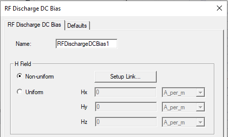
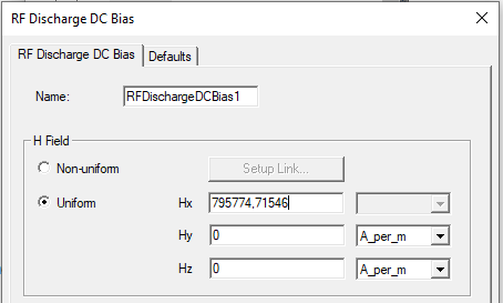
The RF Discharge DC Bias dialog opens. You can specify a uniform bias, or setup a link to a Maxwell project for a non-uniform bias mapped to the selected region.
For example, in the following figure, the region is assigned a uniform magnetic bias of one Tesla (T). The conversion is through Bx (T) = μ0 (Tm/A) Hx (A/m), where μ0 = 4π x 10-7 is the free space permeability.
You can also assign a nonuniform magnetic bias through Maxwell link where the solution of the linked Maxwell project is mapped to the selected region in the RF discharge simulation.
Run RF Discharge Simulation
Once the analysis setup has been completed and the magnetic bias has been added, click Analyze to run the RF discharge simulation.
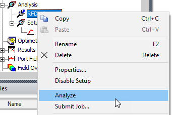
The Frequency Sweep will run first, then the RF Discharge simulation. You watch these occur through the Progress window. At completion, a message appears in the Message window.
Create an RF Discharge Report
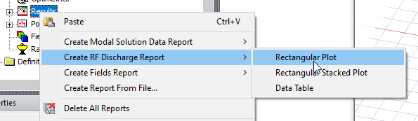
Right click on the Results icon and select Create RF Discharge Report and the type of plot.
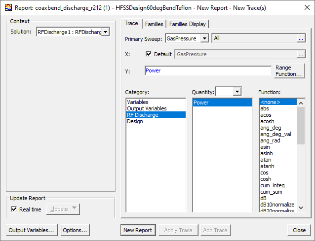
The Report dialog opens up. Select RF Discharge as the Category and Power as the Quantity.
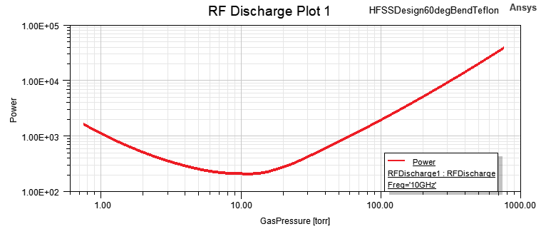
The Paschen curve shown in the plot represents the breakdown power as a function of the gas pressure. In this example, circuit designers mainly care about the minimum breakdown power and the critical pressure where the coaxial bend is most prone to microwave discharge during satellite launch or spacecraft re-entry.
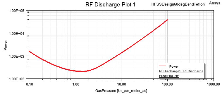
For an eigenmode solution, the breakdown stored energy is equal to the breakdown power divided by the eigen frequency.
(Optional) Change the Pressure Unit
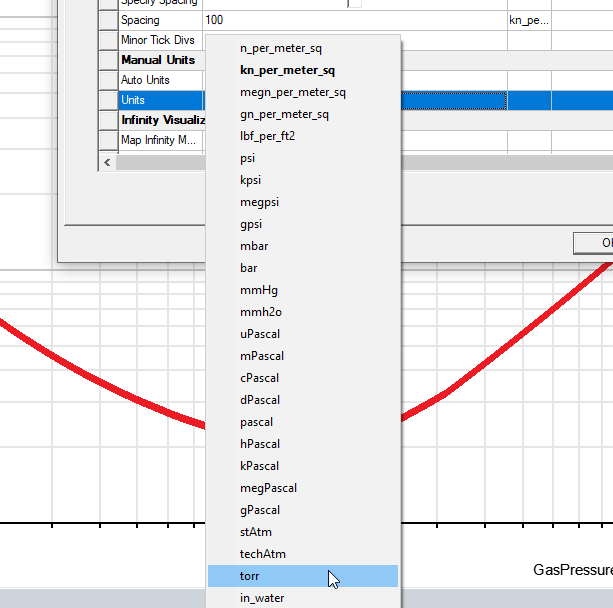
To change the pressure unit, double click Curve Info to open the Properties dialogue and select the X Scaling tab.
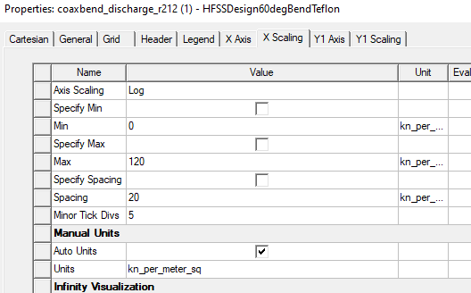
Uncheck Auto Units and on the Units line, use the drop-down menu to select torr.
The plot will become the following by adjusting the bounds of X and Y values to fit the curve in the window.
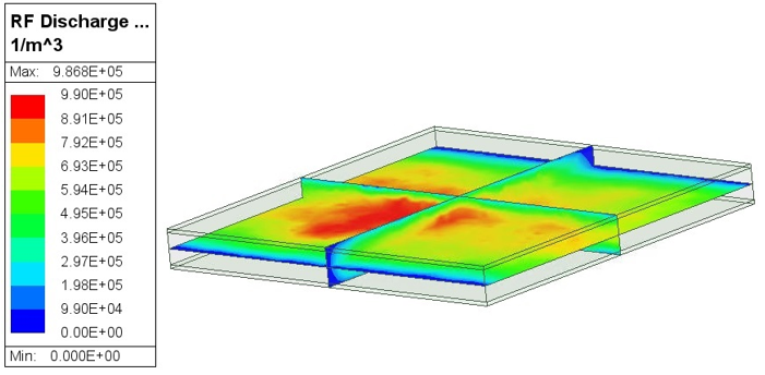
Create an Electron Density Plot or the RF Simulation
Enable the data for an electron density plot in an RF Discharge Analysis Setup checking Save electron density.
 \
\
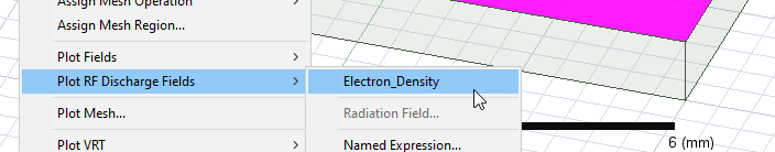
After you solve with this checked, select a face of the object for which you want to plot fields. Then right-click in the Modeler window and select the enabled Plot RF Discharge Fields>Electron Density menu.
Specify parameters in the Create Field Plot window.
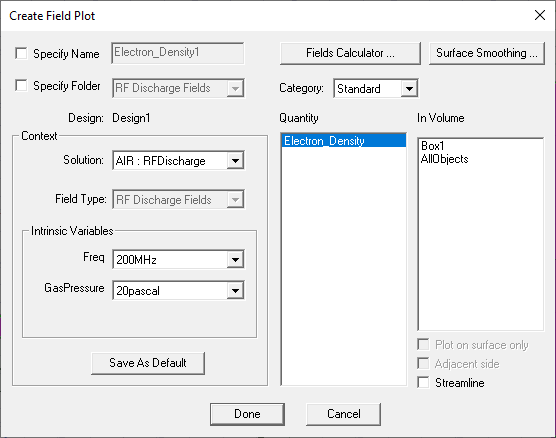
Make Variable and In Volume Selections and click Done.
You can also create an electron density plot for an Eigenmode simulation.
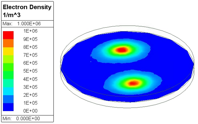
For getting smoother electron density plots, it is often required to use mesh seeding to increase uniformity and density of the mesh. With an increasing mesh density, we can select low order basis functions in Mesh/Solution Options to save simulation time.