Gradient Model for Surface Roughness

The gradient model was proposed by G. Gold and K. Helmreich in reference [1] below. In their approach, random variations in a rough metal surface are modeled by an assumed probability density function (PDF). The PDF describes how likely it is that the surface will be perturbed by some distance above or below its mean height (see Figure 1). Provided that these perturbations are small compared to the wavelength, their effects on a propagating signal can be averaged out. This averaging results in a spatially varying conductivity that is a function of the distance from the mean surface (see Figure 2). This conductivity can be plugged into a one-dimensional version of Maxwell’s equations which can then be solved to yield the effective surface impedance.

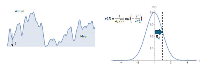
Figure 1: A Rough Suface described with a Gaussian Probability Density Function

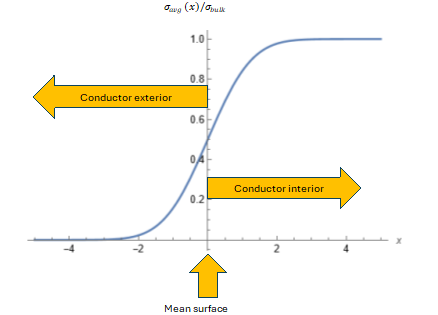
Figure 2: The Spatially Varying Conductivity, σ(x) obtained by averaging the PDF.

An advantage of this approach is that the PDF can usually be characterized by a single parameter, the RMS roughness. This is convenient because the RMS roughness is typically measured by manufacturers and reported on their data sheets.

The gradient model in HFSS supports two types of PDF: Gaussian and Rayleigh. The Gaussian PDF is suitable for a low-profile conductor. The Rayleigh model produces somewhat higher losses and may be more appropriate for a high-profile conductor (see reference [2] below).

References

[1] G. Gold and K. Helmreich, “A physical surface roughness model and its applications,” IEEE Trans. on Microwave Theory and Techniques, vol. 65, no. 10, Oct. 2017.

[2] D. N. Grujic “Simple and accurate approximation of rough conductor surface impedance,” IEEE Trans. on Microwave Theory and Techniques, vol. 70, no. 4, April 2022.