Finite Array Beam Angle Calculator Toolkit

The Finite Array Beam Angle calculator provides:

• An interface to calculate the phase shifts along the A and B vectors of the array lattice, given the scan angles for array elements.
• A script as a template for referencing when writing their own scripts to add functionality and automations.
• Post processing variables for driven and design variables for composite data types for all the data fields to allow you to adjust and modify parameters outside the calculator interface and view corresponding results.
• An interface to calculate different types of tapering, such as triangular, cosine, hamming window, and so forth, and apply these tapering and phase angle to each individual source in the form of either equation or calculated value. You can choose to calculate the taper weights in different coordinate systems, like lattice coordinate, absolute XY coordinates and absolute distance, and visualize the result in an intuitive color map. You can apply tapering to the sub-array and create source groups for the sub-array.

To access the calculator click HFSS>Toolkit>Update Menu. This causes the Toolkit menu to display the Finite Array Beam Angle.

1. To use the calculator, you must first load a project that includes a finite array. The design must have at least one port defined in order to apply excitations to Edit Sources. Select a suitable design and click HFSS>Toolkit>Finite Array Beam Angle.

This displays the Finite Array Beam Angle Calculator dialog:

The Array Selection area is for the Beta Feature for HFSS Multiple Component Arrays. If the feature for multiple arrays is enabled and multiple arrays exist in the design, each array can be calculated individually. When the feature flag is off, the Array Selection control box still appears but only one array can be selected.

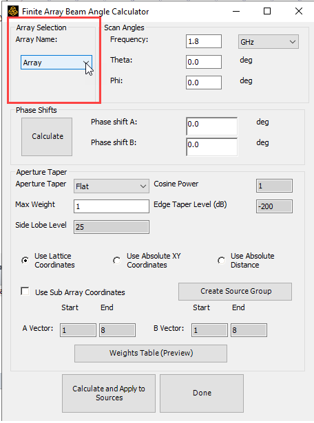
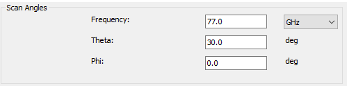
The Frequency field is automatically populated based on the current frequency value.

2. You enter values for Scan Angle Theta and Phi in degrees.

   

   Once you give the scan angle inputs, use the Phase Shifts panel to calculate the phase increment between each adjacent unit cell.

3. Click the Calculate button.

The Phase shift A and Phase shift B fields display the results. If the fields do not initially display, you can size the Toolkit dialog to show all of the necessary digits.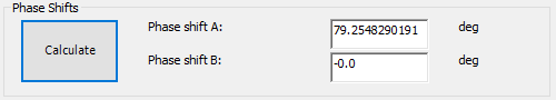

4. Click Calculate and Apply to Sources.

   

5. The Aperture Taper panel contains everything needed to apply taper to each unit cell and create a subarray source group.
   
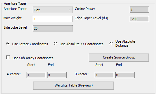
   The Aperture Taper dropdown menu lets you select a tapering method: Flat, Cosine, Triangular, and Hamming Window, Dolph-Tchebychev, Taylor, and Binomial.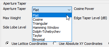
   
   Depending on the method, some variables applicable to the selected taper will become editable on the right side, and you can edit them as they wish.
6. Max Weight allows you to input the largest magnitude for the unit cells. The Max Weight value occurs at the middle of the array and tapers off at the edges.

7. The three radio buttons below the Max Weight text box lets you choose the coordinate system used to calculate weights. The detailed calculation for each tapering method in each coordinate system is described in detail in the next section of this document.

8. Use Sub Array Coordinates allows the user to only choose specific parts of the array to apply weights and phases to.

9. The Create Source Group button creates a source group with the cell within the Sub Array Coordinates. To use the button, you must check the Use Sub Array Coordinates checkbox.

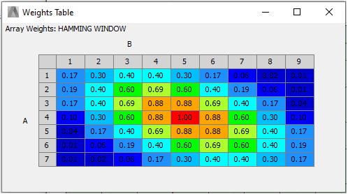
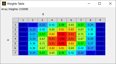
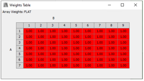
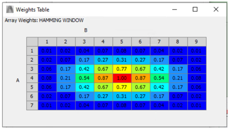
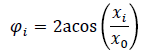
10. The Weights Table (Preview) button displays a color map table that gives a preview of the magnitudes that will be applied to each cell. For example:
    

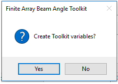
11. Once you have specified all options, click the Calculate and Apply to Sources button. A message box asks if you want to save all results as variables [Yes] or as numeric values [No].
    
    

12. Click HFSS>Design Properties to view the local variables. Scroll down if necessary to view the newly created variables.

    

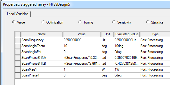
These include ScanFrequency, ScanAngleTheta, ScanAnglePhi, ScanPhaseShiftA, and ScanPhaseShiftB.The values for ScanPhaseShiftA and ScanPhaseShiftB will be expressions. There will also be ScanMagN and ScanPhaseN, depending on the number of modes/terminals.

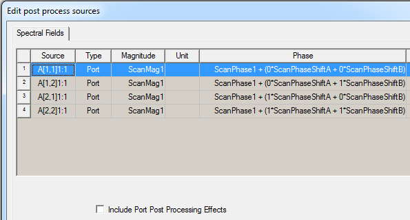
13. Right-click Excitations>Edit Sources to view the Edit Post Process Sources dialog to view the expressions for each source:

    

14. You can then click Radiation>Insert Far Field setups for 3D or XY Plots as needed, and then use Results>Create Far Fields Report to define plots.
15. After you run Analyze and evaluate the plots you create. You can then change the Frequency, the Theta and Phi values, and the ScanMag and ScanPhase variables to see the effects of your changes.

Phase and Weight Calculations

Phase Increment

The phase for a unit cell is calculated by first finding the phase increment between each adjacent cell in both the a and b lattice directions.

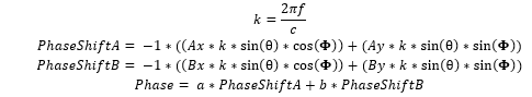
This uses the x and y values of the lattice vectors Ax, Ay, Bx, and By as well as the scanning angle θ and Φ. The variable f is the frequency and c is the speed of light. Then, the phase is assigned depending on the a and b array position.

Aperture Taper Weighting Scheme

Calculating Array Center

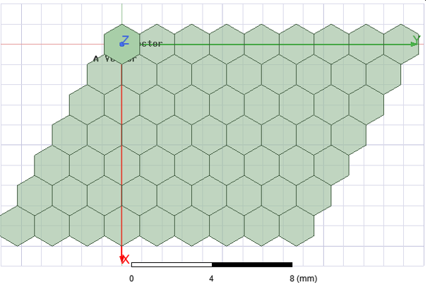
The array center is calculated by first finding the maximum and minimum lattice coordinates in both A and B vectors among all cells. Then, the lattice coordinates of the center of the array is calculated by taking the midpoint between the maximum and minimum coordinates. Finally, the global x-y coordinates of the center of the array is calculated by converting the lattice coordinates into global coordinates.

The example weights table is applied to the following array design:

Lattice Coordinate

For lattice coordinate, the final weight is calculated as Max Weight * W(a,b), where W(a,b) depends on the chosen aperture taper weighting schemes.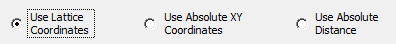

1. Flat:

W(a,b)=1

Weights Table (Preview) for a 7x9 hexagon array:

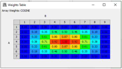
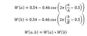
2. Cosine:

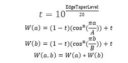
where EdgeTaperLevel is given by user, n is Cosine Power, variable a and b is the index difference between the current cell and the center of the array in lattice A and B vector direction, variable A and B is the maximum index difference among all cells in the lattice A and B vector direction.

Weights Table (Preview) for a 7x9 hexagon array:

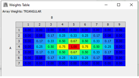
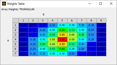
3. Triangular

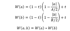
All variables are defined in the same way as those in the previous method

Weights Table (Preview) for a 7x9 hexagon array:

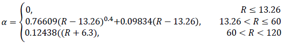
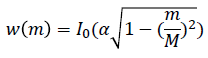
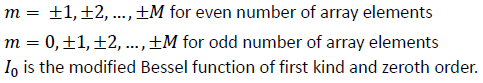
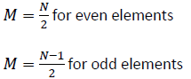
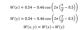
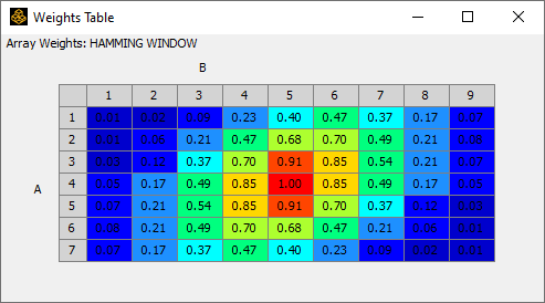
4. Hamming Window

Weights Table (Preview) for a 7x9 hexagon array:

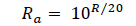
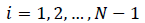
5. Dolph-Tchebychev

	Sidelobe level in absolute units		R is the side lobe level
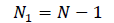
	Number of pattern zeros		N is the number of array elements
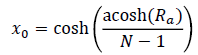
	Scaling factor
	N1 zeros of Chebyshev polynomial
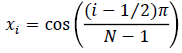
	N1 array pattern zeros in psi-space
	N1 zeros of array polynomial

Weights Table (Preview) for a 7x9 hexagon array:

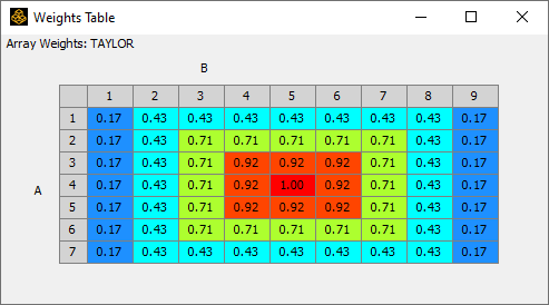
6. Taylor

	Relative sidelobe level in dB (13<R<120):
		R is the side lobe level
	Row vector of array weights:
		N is the number of array elements

Weights Table (Preview) for a 7x9 hexagon array:

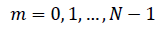
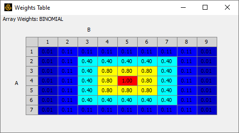
7. Binomial

	Row vector of array weights:

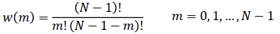
Absolute Coordinate - XY

For absolute coordinate, the final weight is calculated as Max Weight * W(x,y), where W(x,y) depends on the chosen aperture taper weighting schemes. For this selection Dolph-Tchebychev, Taylor, and Binomial are disabled.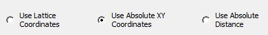

1. Flat:

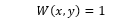
2. Cosine:

where x and y are the distance between current cell and the center of the antenna array in global x-y coordinate. X and Y are two times the longest distance between the edge of the array and the center of the array in global x-y coordinate.

Weights Table (Preview) for a 7x9 hexagon array that is aligned with global x-y coordinates:

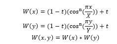
3. Triangular

Weights Table (Preview) for a 7x9 hexagon array:

4. Hamming Window

Weights Table (Preview) for a 7x9 hexagon array:

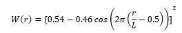
Absolute Coordinate - Distance

For absolute coordinate, the final weight is calculated as Max Weight * W(r), where W(r) depends on the chosen aperture taper weighting schemes. For this selection Dolph-Tchebychev, Taylor, and Binomial are disabled.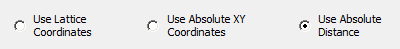

1. Flat:

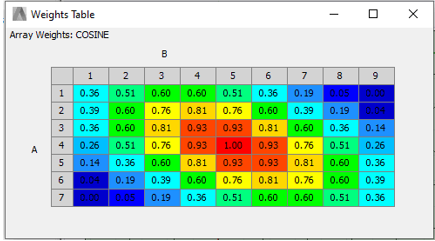
2. Cosine:

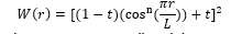
where r is the absolute distance between current cell and the center of the antenna array, and L is two times the longest distance between the edge of the array and the center of the array.

Weights Table (Preview) for a 7x9 hexagon array:

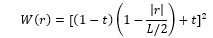
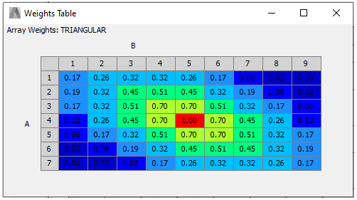
3. Triangular

Weights Table (Preview) for a 7x9 hexagon array:

4. Hamming Window

Weights Table (Preview) for a 7x9 hexagon array: