
OptimTee
Abstract
This model demonstrates the optimization of a waveguide T-junction operating over a frequency range of 8-10 GHz. A septum splits and steers the input signal between two output ports. A design variable controls the position of the septum.
This example model is installed with the Ansys Electronics Desktop software and is located as follows:
<installation_path>\ANSYS Inc\v252\AnsysEM\Examples\HFSS\RFMicrowave\OptimTee.aedt
Solution Time: 12 cores, Intel Xeon Gold @ 2.9 GHz, in version 2025 R2
Real Time: 00:01:35, 213 MB max. RAM
(adaptive solution, frequency sweep, parametric sweep, and optimization)
Description
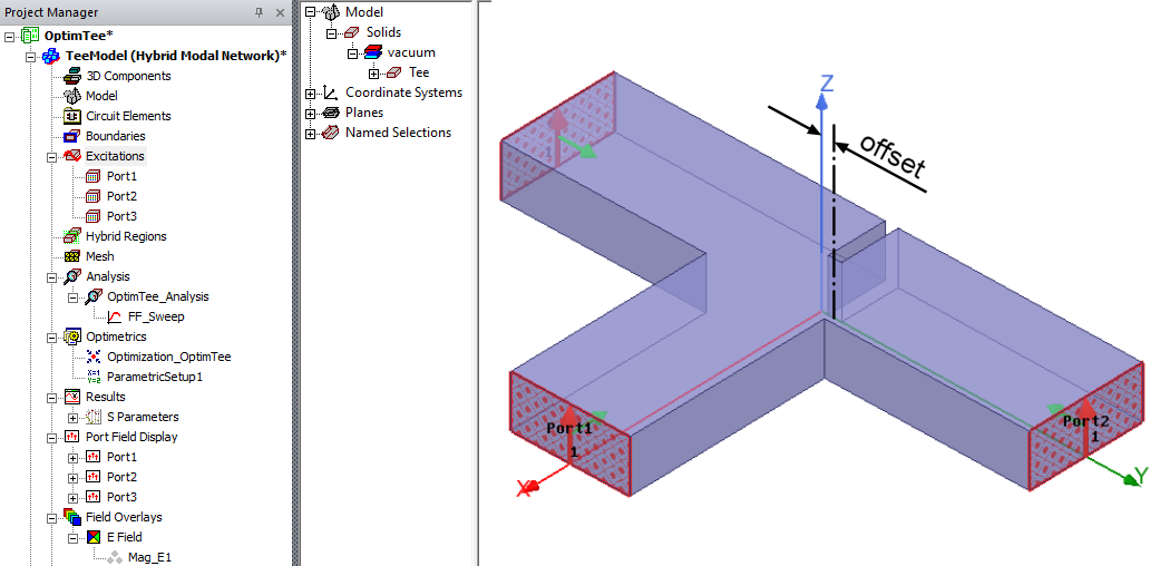
The T-Junction is a simple power divider that might be used in a feed network. The septum position determines how the input power on Port 1 splits between Ports 2 and 3. The arms are a standard X-band waveguide, and the location of the septum is controlled by a design variable (offset). The septum offset is initially set to 0.1 inch.
Related Getting Started Guide:
In addition to the example project, the following getting started guide is based on the same device and provides you the opportunity of building the geometry, setting up the analysis, solving, and postprocessing the results on your own:
Getting Started with HFSS: Waveguide T-Junction Optimization
The solution setup and the results postprocessing are not necessarily identical between the example model and the getting started guide.
Model and Simulation Setup
This model is a single, vacuum-filled solid with ports assigned to the three faces, as shown in the preceding figure. The default boundary for the other outer faces is PEC. This model is set to adapt at 10 GHz with an interpolating frequency sweep from 8 GHz to 10 GHz. You can change the value of the design variable, offset, by clicking HFSS > Design Properties.
To view a port or boundary, select the desired item in the Project Manager. The relevant item is highlighted in the Modeler window, and the properties are displayed in the docked Properties window. Selecting an object in the History Tree also displays its properties.
In addition to the interpolating frequency sweep, there is a parametric sweep predefined. It solves for variants of the septum position ranging from offset = 0 inch to 1.0 inch in 0.1 inch increments.
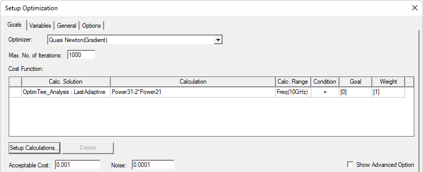
Finally, an optimization is predefined with the goal of determining the offset value at which the sum of the power flowing from Port 1 to Port 3 equals twice the power flowing from Port1 to Port2 (within a 0.001 stopping criterion). Output variables are defined for ease of setup. The parametric sweep is run automatically before the optimization is performed. The following figure shows the optimization setup:
To run the adaptive solution, frequency sweep, parametric sweep, and optimization using a single command, right-click Tee Model (Hybrid Modal Network) in the Project Manager and choose Analyze All from the shortcut menu.
Postprocessing
Once the model is solved, the solution data can be viewed by right-clicking OptimTee_Analysis and choosing Profile. The Solutions dialog box appears. Tabs are included for Convergence, Matrix Data, and Mesh Statistics.
To view a plot of S parameter data, look in the Project Manager under Results, and double-click S Parameters.
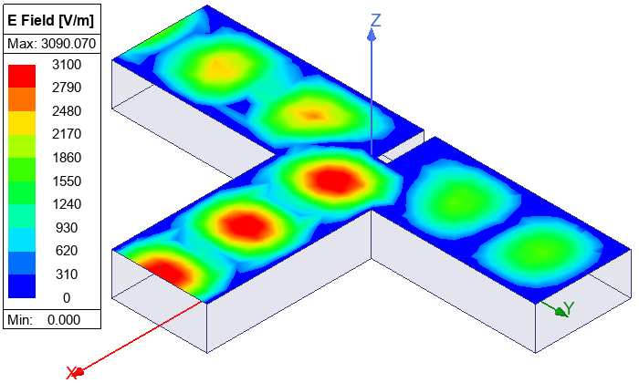
To view the E field plot (shown below), double-click Mag_E1 under Field Overlays > E Field. A phase animation of the E field can be plotted by right-clicking Mag_E1 and choosing Animate. Then, click OK in the Create Animation Setup dialog box and click Animate.
Additionally, you can view an offset animation of the E Field to see how the field distribution changes as the septum is moved, as shown below:
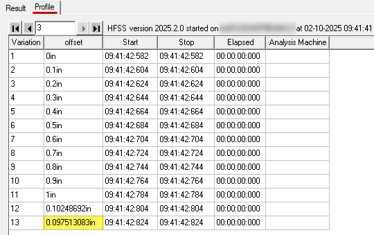
View a table of the optimization results by right-clicking Optimization_OptimTee (under Optimetrics in the Project Manager), choosing View Analysis Results, and selecting the Profile tab. This table appears in the following figure:
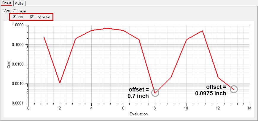
Select the Plot option under the Results tab. Also, select Log Scale for better resolution at the low end of the Y scale. The plot shows two offsets that satisfy the target power ratio within the specified Acceptable Cost (stopping criterion) of 0.001:
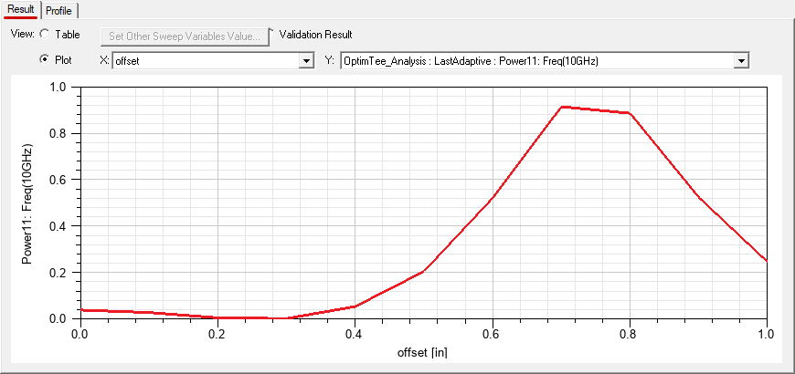
If you look at an offset animation of the E Field, you can see that signal reflection at Port1 is high, and throughput to Port2 and Port3 is very low, at offset = 0.7 inch. Addtionally, right-click ParametricSetup1 (under Optimetrics in the Project Manager) and choose View Analysis Result. In the Results tab, you can choose to see a plot of Power11, Power21, or Power31 versus offset. The following figure is the Power11 plot, which shows very high signal reflection at Port1 for offsets greater than 0.5 inch. Signal reflection for offsets equal to or less than 0.4 are low. Clearly, 0.0975 inch is the optimal offset value among the two that satisfy the power ratio goal.
Finally, you can view the source fields by selecting Port Field Display > Port1 > Mode 1 In the Project Manager. Right-click on this entry and select Zoom to Region to enlarged the vector plot of the TE10 mode on Port1 so that it fills the Modeler window.