Gregorian Reflector

Abstract

This example shows a comparison between the solution of a Gregorian Reflector antenna using the hybrid FEBI-IE and the hybrid FEBI-IE-SBR+ approaches in HFSS.

Solution Time: 16 cores Xeon Gold @ 2.9 GHz, single Nvidia GPU, in version 2025 R2
(meshing, adaptive solution(s), and other options as detailed below)

Design Name: Setup Description	(*)	Skip IE Region?	Skip SBR Region?	Time	Max RAM (GB)
IE_Regions: Hybrid FEBI-IE	1	No	N/A	29m 33s	5.22
IE_Regions: Hybrid FEBI-IE	2	Yes	N/A	28m 58s	5.27
IE_SBR: Hybrid FEBI-IE-SBR+	3	Yes	Yes	3m 42s	0.783

Note:

Simulation time and memory will vary depending on your available resources. In most cases, HPC (parallel resources) can be leveraged to significantly reduce simulation time and the memory footprint required by each CPU.

For both designs, the option to Skip ID Region Solve During Adaptive Passes for FEBI is found under the Hybrid tab of the Driven Solution Setup dialog box. The option to Skip SBR+ Solve During Adaptive Passes is only applicable to the second design. It also is located under the Hybrid tab of the Driven Solution Setup dialog box but is selected by default and cannot be altered. That is, SBR regions are always skipped during the adaptive solution.

(*) Rows 2 and 3 represent the active configurations of the IE_Regions and IE_SBR designs, respectively, in the Gregorian_Reflector project file.

Description

HFSS SBR+ can provide significant time and memory savings for computing large reflector electromagnetic interactions. Most asymptotic solvers hybridize only to Method of Moments/Integral Equation (MoM/IE) solvers. However, HFSS supports hybrid solutions combining SBR+, Finite Element (FEM), and/or IE methods in a single design. Specifically, an HFSS design with an SBR+ Region can also include Finite Element–Boundary Integral (FEBI) and IE Regions. FEBI or IE Regions may or may not have electromagnetic source excitations assigned.

In this example, all full-wave regions are first pre-computed then applied to SBR+ regions. All full-wave regions (FEBI, IE) are considered independently. In practice, closely spaced (near field) full-wave regions should be grouped so that their 2-way couplings are considered prior to hybridization to an SBR+ region.

The model is a 10 GHz Gregorian reflector system with two predefined HFSS designs, set up as follows:

In both designs, the horn is set to FEBI, defined within a 3D component, and the sub reflector is set as an IE Hybrid Region.
In the first design (named "IE_Regions"), the large reflector is also set as an IE Hybrid Region.
In the second design (named "SBR_Region") the large reflector is changed to an SBR+ Hybrid Region.

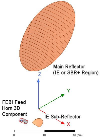
Gregorian Reflector model including feed horn, sub reflector, and main reflector

Full-wave solvers, such as FEM and IE regions, should be utilized for closely coupled structures, such as the sub-reflector and feed horn.

Horn: HFSS FEM (FEBI boundary)
Sub-Reflector: IE Region

The main reflector can also make use of FEM or IE solvers or, alternatively, ray-tracing and physical optics methods (SBR+, PO), which can speed up the simulation dramatically.

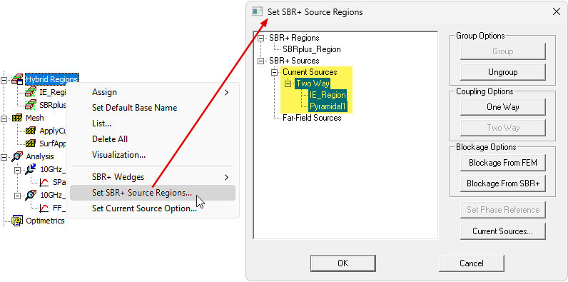
Set Two-Way interactions for full-wave hybrid regions. By default, full-wave regions will operate on the SBR+ region independently. We want the FEBI (Pyramidal Horn 3D Component) and IE Regions to be simulated as coupled before applying them together to the SBR+ region.

Right-click on Hybrid Regions and select Set SBR+ Source Regions.
Make sure the FEBI and IE Regions are grouped under Two Way sources.

Hybrid Regions shortcut menu showing how to access the Set SBR+ Source Regions command and also showing the settings in the resulting dialog box

The IE_Regions design has one solution setup and a frequency sweep (Sparam_Sweep). It is an interpolating sweep ranging from 9.2–10.8 GHz in 100 points).

The IE_SBR design has two solution setups (10GHz_2D_pattern and 10GHz_3D_pattern). Only the 2D solution includes a frequency sweep (Sparam_Sweep), which is identical to that of the IE_Regions design. Under the Hybrid tab of the Driven Solution Setup dialog box (for designs with SBR+ regions), you must specify the Field Observation Domain (2D or 3D in this case). For this reason, there must be two separate solution setups when you plan on postprocessing SBR+ results in two different observational domains. For efficiency, and to improve the solution time, the 2D solution imports the mesh from the 3D solution, forcing the 3D solution to be solved first. All reports where the result is plotted versus frequency are derived from the 2D solution.

Mesh Operations:

Each design includes the following two mesh operations:

ApplyCurvilinear1 – Enable curvilinear meshing for the small and large reflector objects.
SurfApprox1 – Specify a maximum surface deviation of 0.15 mm and a maximum aspect ratio of 2 for the small and large reflector objects.

Based on the 10 GHz adaptive solution frequency, 0.15 mm equals λ/200, which is a good allowable surface deviation guideline for models similar to this example.

Postprocessing and Simulation Comparison

Comparing the first design results (using FEBI and IE Regions) with the second design results (using FEBI, IE, and SBR+), there is excellent agreement. To directly compare the results, copy the data from the second design's 2D_Radiation_Pattern plot and paste it into the first design's 2D Radiation Pattern plot. Then, set the color of the second design's trace to green and set the red and green traces' line widths to 2 and 1, respectively, so that you can see both traces clearly, as shown in the following figure:

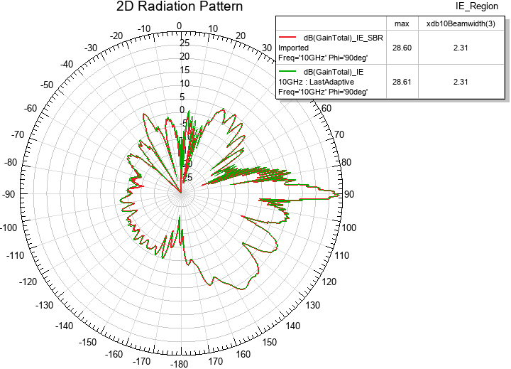
2D radiation patterns, comparison of first design (FEBI IE) and second design (FEBI IE SBR) results showing excellent agreement

Using SBR+ for the main reflector reduces the overall simulation time significantly, as seen in the preceding Simulation Time table. Reduction grows exponentially with the electrical size of the problem. SBR+ makes it practical to simulate installed sidelobes for antenna system and its host platform (satellite payload, etc.)

A hybrid analysis can also benefit from skipping IE regions during the adaptive analysis. Enable this option in the relevant analysis setup. Refer to the preceding Simulation Time table to see the effects of this option. Note that SBR+ regions are always skipped during the adaptive solution.

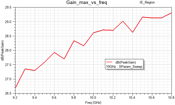
The following figure is the maximum gain versus frequency for the IE_Regions design:

Maximum gain versus frequency plot for the IE Regions design

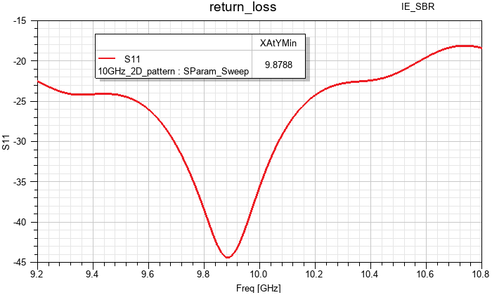
The following figure is the return loss versus frequency for the hybrid IE_SBR design:

Insertion loss versus frequency plot for the hybrid IE SBR design

Finally, 3D gain plots are predefined for both designs. Additionally, there is a stacked plot in each design showing total gain versus theta at three frequencies (9.2, 10.0, and 10.8 GHz). Double-click any of these reports, under Results in the Project Manager, to open and review the plots of interest.