How to Check Causality, Passivity & Fitting Error

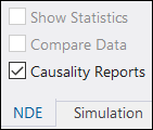
Use Network Data Explorer (NDE) to view the aspects described in Section III., such as the quality of data fitting. Upon reviewing the exported S-parameter data in NDE, review the causality of the data when it is exported into a macromodel (i.e., state space model) by clicking Broadband in the top ribbon of NDE (shown in the following screenshot).

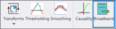
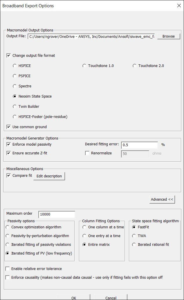
Once the default settings and format are selected for a Nexxim state space model, generate the macromodel via the Broadband Export Options window.

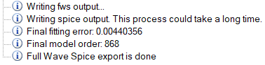
Once the macromodel is generated, the final fitting error will be displayed in the Message Manager window (shown in the following screenshot).

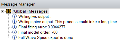
In this example, the final fitting error is 0.0044277 or approximately 0.44%. The macromodel is causal with respect to the fitting error tolerance of 0.5% set during export. The final fitting error could potentially exceed 0.5% which would mean, with a threshold of 0.5%, that the macromodel is not causal. The tolerance could also be altered (e.g., set to 0.1%, 1%, etc.) for double-checking the causality of a macromodel with tolerances lower and higher than the default 0.5%. Sometimes, tightening or loosening the tolerance gives a better fit. The latter works because a lower (i.e., tighter) fitting tolerance, the software may try to over fit the data and, in the process, destroy the fitting quality of the macromodel. This could result in, for example, many (out of band) passivity violations.

The following screenshot demonstrates one method for checking causality.

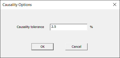
This method yields a colored plot (following). The data is causal, non – causal, or inconclusive.

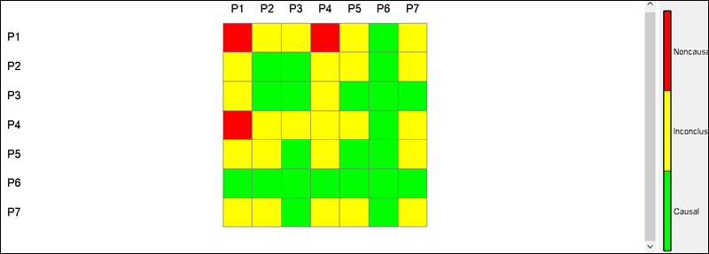
Note that the colored plot is also generated with respect to the tolerance set by the user (in this case, the default fitting error is 2.5%). There is no direct correlation between the tolerance of 2.5% here and 0.5% fitting error set in the Broadband Export Options window. Use this example for guidance, to see where the data is not meeting causality once the fitting error check returns a bad result. This example should not be used as a final basis to check for causality. Once the macromodel is created and returns a satisfactory causality check result, it returns to the Broadband Export Options window.

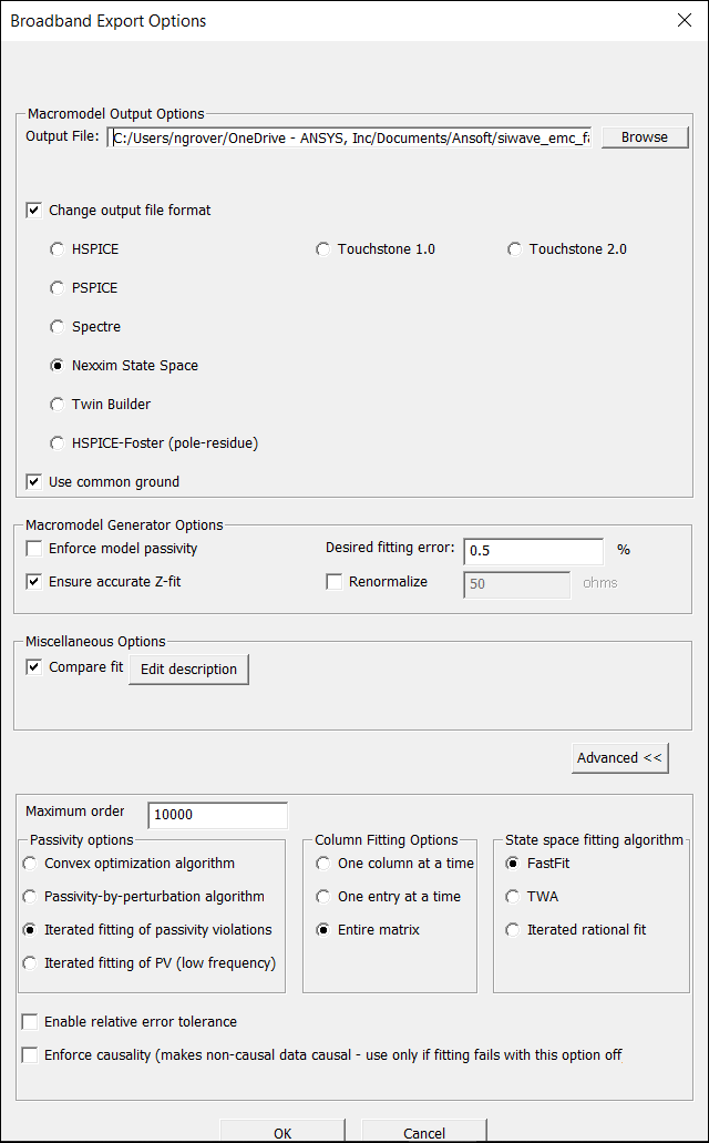
This time, check the Enforce model passivity box and select Iterated fitting of PV (low frequency) from the Passivity options group box (i.e., IFPVLF), as shown in the following screenshot.

Once the new macromodel is generated, the final fitting error will appear again in the Message Manager window. Fitting error (with IFPVLF considered) will be displayed as in the following screenshot.

If the error is below the fitting tolerance of 0.5%, the generated macromodel is causal and passive. Subsequently, the macromodel can be utilized for the next step of transient simulation. A final fitting error below the fitting tolerance is a necessary condition for a good fitting experience but may not be sufficient when generating a broadband macromodel for a transient simulation. It must be ensured that the transient simulation functional output makes sense.

Consider that though the original S-parameter data may be causal and passive, there is no guarantee that the resultant macromodel is going to remain passive. For example, assuming the user has the following data: 1.0, 1.0, 0.9999, 0.9999 and so on, at several frequency samples, and a rational fit is applied to this data, given that the data is causal and passive, and the target fitting error is 0.5% or 0.005. The resulting fit would be: 1.0049, 1.0049, 1.00001, 1.000001 and so on. Though the fitting error is better than 0.5%, the maximum singular value is 1.0049, which exceeds one. Hence, the result is non-passive. Though the data is causal and passive, the fit may not be.

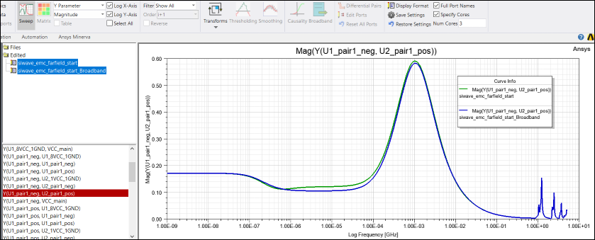
What is important is what the macromodel fitting tool does with respect to the original S -parameter data. This can be done in NDE, using a “Y” parameter plot in magnitude (with log – log axis), as shown in the following screenshot. The green line is the original data, and the blue line is the fitted data: