
Advanced Settings for Characterizing a Power Diode
Click Adv. Settingsin the Dynamic Model Input [6/8] dialog box to access advanced settings of power diode characterization. There are two tabs: Extraction Settings and Model & Goal Settings.
- Extraction Settings
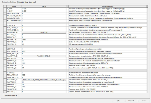
Advanced Parameter Setting Dialog Box
These settings allow for more control over the characterization process, but it should not be necessary to change them for most devices. The diode model used for characterization also appears as a sub model of the dynamic IGBT and MOSFET models.
|
Parameter |
Information |
||||||||||||||||||||||||||||||||
|
H_ON and H_OFF |
H_ON and H_OFF are the initial settings for the On-switch and OFF-switch signal acquisition times. The actual Hon and Hoff values change during the characterization. Hon and Hoff derive from the measured switching times and length of the reverse recovery. 5x…10x of the On-switch/reverse recovery time should be a good value. For SiC devices the values should be much smaller than for Si devices. If the initial values are not good, the extraction process will not be able to determine the sensitivity of parameter changes to the output signal and the extraction will not start to converge. You can observe the convergence of the extraction on the Fitting info page and adjust the initial values for H_ON and H_OFF if necessary. |
||||||||||||||||||||||||||||||||
| INTEGRATION | Integration method (0 is best for switching devices). | ||||||||||||||||||||||||||||||||
|
MEASURE_FLAG |
Measurement mode (1 allows for stop of measurement cycles as soon as a good result is reached). |
||||||||||||||||||||||||||||||||
| MEASURE_REPORT | Measurement tool output (should stay 1). | ||||||||||||||||||||||||||||||||
| FITTINGREPORT | Fitting report output (should stay 1). | ||||||||||||||||||||||||||||||||
|
LOOPS_A, LOOPS_B, and LOOPS_C |
Approaching the optimal parameter set is an iterative procedure. This iteration is split into three sequenced loops: A, B, and C. Each sequence can repeat any number of times according to LOOPS_x. This is especially helpful in the case of loop A, which is a predefined sequence of one dimensional parameter sweeps. In some special cases an increased number LOOPS_A can result in much better initial parameter values before starting the Newton-Raphson-based matrix loops B and C. Default values are LOOPS_A:=0, LOOPS_B:=1 and LOOPS_C:=1. |
||||||||||||||||||||||||||||||||
|
MASK_PAR_A |
This is a list of dynamic model parameters which take part in the 1D parameter sweep sequence. The input is interpreted as a parameter mask for parameter selection during the characterization.
A repeated application of loop A helps to find a good initial parameter guess for the following Newton-Raphson-based loops B and C. The above table also shows the most likely parameter-to-goal impact which is useful in case of manual parameter optimization. If a parameter appears sequenced, then different combined and direct impacts are tested. In some cases diodes are already characterized just after loop A. |
||||||||||||||||||||||||||||||||
|
MASK_PAR_B and MASK_PAR_C |
Lists of dynamic model parameters which take part in the Newton-Raphson-based parameter optimization by error minimization. The following parameters are recognized. The parameters included by default are in bold letters.
|
||||||||||||||||||||||||||||||||
|
NUM_JACO_A NUM_JACO_B, and NUM_JACO_C |
This parameter defines which entries from the sensitivity matrix are considered for the matrix search: -1: largest column, 0:apply threshold >0: this number of largest entries For Loops_A when simple 1D search is used, this parameter is ignored. |
||||||||||||||||||||||||||||||||
|
TOL_JACO_A TOL_JACO_B, and TOL_JACO_C |
This parameter defines the relative threshold for Jacobian entries to be used in the matrix search (when NUM_JACO_x = 0). For LOOPS_A it can be set to -1 which will switch LOOPS_A to simple 1D search. |
||||||||||||||||||||||||||||||||
|
RESORD_A, RESORD_B, and RESORD_C |
This is the order of the residual. The number range is 0 .. 2: 0 – The maximum error is the residual value (the error number). 1 – Absolute error average. 2 – Root mean square error value. To observe the system approaching from far the optimum toward the optimum solution number 2 is best suitable. Finally we claim that every goal value has a smaller error than a certain limit. Here we have to use 0. This is the reason for RESORD_C:=0 in every characterization. |
||||||||||||||||||||||||||||||||
|
RESTOL_A, RESTOL_B, and RESTOL_C |
Desired accuracy of the residual according to the RESORD setting. To quickly move the model parameters toward the optimum, the tolerance can be set as large as 0.2 = 20%. The number of necessary loops A, B and C will decrease strongly. It is suggested to use the final accuracy only in the last main loop (usually loop C). Relaxing the accuracy can result in a noticeable reduction of simulation time. |
||||||||||||||||||||||||||||||||
|
MATRIX_A
|
Within loops A (when matrix search is used) and within loops B and C the recalculation of the Jacobean matrix will be done this number unless the residue falls within the accuracy region. The value for MATRIX_x are the maximum numbers of Jacobean re-calculation, which takes most of the simulation time. In terms of pure mathematics, the recalculation should be done in every iteration cycle to stay close on the direct path to the optimum. It turns out to be a good trade-off between the shortest path and the simulation duration to leave the Jacobean untouched for some iterations before its recalculation by simulation. For Loops_A when simple 1D search is used, this parameter is ignored. |
||||||||||||||||||||||||||||||||
|
ZEROFN_A
|
This is the number of iterations without changing the Jacobean (system) matrix. Only the right side of the balance system—the so-called zero function—is changed in every iteration step. This residue calculation is much faster and drives the parameter changes in roughly the right direction toward the optimum solution (the optimum parameter set). These values are called Samanski factors. For Loops_A when simple 1D search is used, this parameter is ignored. |
||||||||||||||||||||||||||||||||
|
RESLOC_A RESLOC_B, and RESLOC_C |
Numbers of local residue (under-relaxation values differ between parameters) use before the system is considered to become stiff and hard to solve. After RESLOC_x total iterations for under-relaxation and boosting the main diagonal of the Jacobean, no longer is each parameter treated separately but all together globally the same way (under-relaxation values equal for all parameters), which slows down the convergence considerably but forces the solution path back to the optimum path. The additional convergence control stays unused by large RESTOL_x numbers to save time and to make the optimization feasible. For Loops_A when simple 1D search is used, this parameter is ignored. |
 and
and  . The templates are scalable so that very different reverse responses can be modeled.
 marks the transition from exponential current wave at discharging the diffusion capacitance to a sinusoidal approach to the peak current. The range is 0 … 0.995 but zero is the best setting to avoid voltage oscillation at the transition point. R1_D is excluded from parameter optimization.
 of the wave form. It can be smooth transition from cosine to an exponential decay in case of TYPE_FWD:=2 () or a kink in case of TYPE_FWD:=3 (), if the measurements are available. Otherwise, TYPE_FWD:=2 is preferred.
 in the plots
 in to control the softness and thus the voltage overshoot at off switch. Together with R2_D, SF1_D provides additional freedom to fit for TRR, QRR and IRRM together.
 in plots.
 . If the C(V) characteristic is given, you can derive DELTA_C from the curve. If not, the input zero triggers an internal initial guess for this value.
 and thus a combination of displacement charge and excess carrier charge in the free wheeling diode.
- Model & Goal Settings
Use the Dynamic Behavior drop-down list to choose a reverse recovery model. The mapping between the menu options and value of parameter TYPE_DYN is:
| Dynamic Behavior | TYPE_DYN |
| Dyn0 (no reverse recovery) | 1 |
| Dyn1 (+exponential Irr) | 2 |
| Dyn2 (+linear Irr) | 3 |
Description of parameter TYPE_DYN and different reverse recovery models can be found in . Note that in the final characterized model, TYPE_DYN is added by 10 so it takes external synchronization input for accuracy of switching behavior (see TYPE_DYN=x+10 in the detailed documentation). That is why we see value of TYPE_DYN is 11, 12 or 13 in characterized power diodes.
You can choose dynamic fitting goals in Select Goals to Display. The checked goals appear in the table of dialog box Dynamic Model Input [6/8], so it can be included as fitting goals during extraction.