Ansys Icepak Component Interface Concept

Thermal Analysis using a Foster Network

In this method, the thermal problem is treated like a system. A system is an entity that processes a set of inputs and yields another set of outputs. For the thermal problem at hand, the inputs are power (or heat source), and the outputs are the temperature at user-specified locations. When a system is Linear and Time Invariant (LTI), the system has the following features:

The system is completely characterized either by its impulse response or step response.
If two LTI systems have the same impulse or step response, the two systems behave identically in that the outputs of the two systems are the same provided that the inputs to the two systems are the same.

This feature allows a Foster network, which is an LTI system, to represent the thermal system, which also can be an LTI system under certain conditions.

Single input and single output system

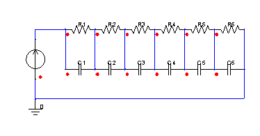
This section describes the simplest system: one with a single input and a single output. The thermal problem is such that the power is from one component, and the output is the temperature at one user-specified location. A Foster network problem for this kind of system is shown in Figure 1, in which the input is the current to the network, and the output is the voltage at the same location.

Foster Network

As mentioned above, both the thermal and Foster systems are LTI under certain conditions; they will behave identically if they have the same impulse or step response. Since the step response is easier to work with, the goal is to match the step response of the two systems. The step response of a typical thermal system is shown in Figures 2 and 3 for self-heating and cross-heating. Note that the self-heating curve has a positive slope at the start of the curve, while the cross-heating curve typically has close to zero slope at the start of the curve.

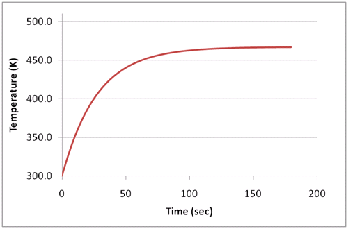
Typical step response for self-heating

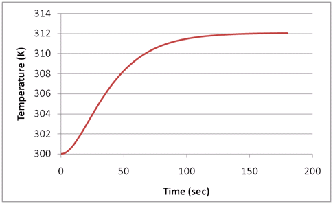
Typical step response for cross-heating

The step response of a Foster network is shown in the following equation:

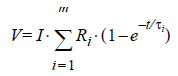
where m is the number of rungs or RC pairs, and parameters R_i and must be extracted through curve fitting the transient step response of the thermal system.

A typical step response from a Foster network will not give close-to-zero slope as required by the cross-heating curves, and thus we cannot match the step response of cross-heating from the thermal system. However, if one allows for negative R, the resistance, the curve fit works well. Even though negative R poses no difficulty mathematically, it causes problems in circuit simulators. You can overcome this difficulty by using positive R but subtracting the V contribution from that part of the RC circuit. Figure 4 shows an example. In this example, the voltage (or output) equals VM1 minus VM2 rather than VM1 plus VM2. So, the Foster network itself has no negative Rs, but rather it has a part with negative voltage contribution.

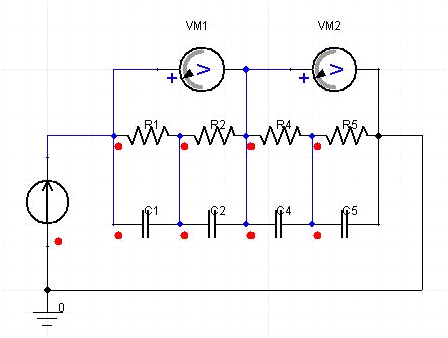
A Foster Network accounting for negative R

As long as the step response from the Foster network matches that from the thermal system, we are guaranteed that the subsequent response from the thermal system under any transient input can be represented by the Foster network, due to the characteristics of LTI systems mentioned in the introduction. Mathematically, if the step response of a system is known, then the impulse response, designated typically by h(t), is known to be the derivative of the step response; and h(t) entirely characterizes the system through the following equation:

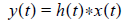
where x(t) is the input, y(t) is the output, h(t) is the impulse response, and * designates convolution. Even though we could use the convolution equation to calculate the thermal response, we choose to use the Foster network to represent the thermal system due to its simplicity to implement in circuit simulators. In passing we note that if the step response is too complex for the Foster network to curve fit, one can always rely on the convolution method. Also, convolution notation makes it easier to express the solution for systems with many inputs and outputs as described below.

Systems with many inputs and many outputs

For systems with many inputs and many outputs, the superposition property is used to obtain the solution. Superposition means that the overall output at one location is the sum of the contribution from individual inputs. The convolution equations satisfy the superposition property. In terms of the impulse response h_ij, the solution for a system with m inputs and n outputs can be calculated using the matrix below:

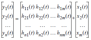
where h_ij represents the impulse response of the jth input on the ith output, and again * designates convolution rather than product. As before, instead of using the convolution method, a Foster network represents the thermal system. But instead of curve fitting one step response, we need to curve fit n×m number of step responses in principle. However, many of the cross-heating responses have very small values, and thus their contribution can be neglected. In passing we note that the Laplace transform of the h_ij represents the impedance between the jth input and the ith output.

Also note that the impulse response matrix would, in general, not be symmetrical even though the system is linear. This is because in a convection heat transfer problem, a downstream object will strongly “feel” the heat from an upstream object but not vice versa. However, there are problems with symmetrical impulse responses, such as diffusions problems with temperature boundary condition.

Limitations and assumptions

As mentioned above, this method works provided that both systems are LTI. The linearity part of LTI means that the system must satisfy the superposition property. The time invariant part of LTI mainly concerned with the coefficients of various terms in the governing equations of the system, which are typically ordinary or partial differential equations. For the Foster network, if the resistance and capacitance are constants, the system is linear and time invariant. We will next discuss under what conditions thermal systems are LTI.

Thermal problems, governed by Navier-Stokes equations, are, in general, notoriously non-linear. So thermal systems processing power inputs and yielding temperature outputs are in general not linear. The linearity is mainly due to, but not limited to, the momentum equation. However, if density and properties are constant, the momentum equation is decoupled from energy equation. This decoupling makes the energy equation linear and thus the thermal systems linear. But as mentioned above, the thermal system needs to be time invariant as well. To make the thermal system time invariant, the coefficients of all terms in the energy equation need to be constant. Flow velocity, which serves as the coefficients for energy equation in the convection term, is the main concern. So, in order for the system to be time invariant, velocity cannot change as a function of time even though no restriction is applied on spatial variation.

The thermal system can also be linearized by choosing the properly operating point. However, this method has limited application for thermal systems as linearization requires that heating has a large DC component and relatively small variation superposed onto it. Most thermal problems do not satisfy this condition. However, if this condition is satisfied, the Foster network method is valid.

To summarize, the following conditions must be satisfied in order for the thermal system to be LTI and thus make the method valid:

Constant density – This is a very good assumption for incompressible fluids like water. For compressible fluids like air, constant density implies low Mach number and adiabatic temperature boundary condition. Even though the low Mach number condition does not pose real restrictions on most of problems considered, the adiabatic temperature boundary certainly cannot be satisfied strictly for heat transfer is the main point of interest. However, testing shows that the method still gives very decent results even when the max temperature increase goes up to 140K.
Constant property – This is not a major concern as the properties either do not change appreciably within the range of temperature, or the impact of the property is rather negligible. Density variation will likely show signs of a problem before properties variation.
Constant velocity – The Foster network, characterized at one velocity, cannot be used for other velocities. A new characterization (curve fitting) is needed if velocity changes.
No radiation – This restriction is due to the non-linear relationship between temperature and radiation heat flux.

Foster network and thermal network

Before concluding the discussion, it might be worthwhile to talk about the difference between the current Foster network method and a traditional thermal network. In the traditional thermal network, the thermal problem is represented by thermal resistors and thermal capacitors. To obtain the model parameters, no curve fitting of step (or impulse) response is typically performed; the parameters can be extracted from various methods, ranging from physical argument to testing. The thermal network method is not limited to linear systems, even though it is applied most successfully to such a system. Another important difference is that in a thermal network each node represents a physical location, while in the Foster network it is noted that only the input and output nodes have physical connections; the rest of the nodes in the Foster network have no physical significance. Finally, the Foster network has the advantage of being more accurate provided the conditions are satisfied because the results from the Foster network are as accurate as the method generating the step (or impulse) response.

In summary, the thermal network is more general with perhaps compromised accuracy; while the Foster network is more accurate but with more restrictions attached to it.