Introduction

This topic reviews a few basic concepts from electromagnetics and circuit theory that are essential to this discussion.

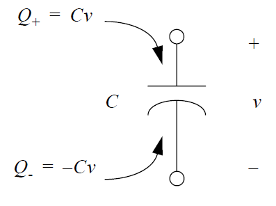
Two-Terminal Capacitor

A two-terminal capacitor of value is shown in the figure below, with the charges on the top and bottom plates shown. below. Recall from basic circuit theory that each "plate" of the capacitor has associated with it a certain charge. The "top" plate (the one that serves as the positive reference for the branch voltage ) has a total charge spread over it. The bottom plate has an equal and opposite charge . The charges are always equal and opposite because it is assumed that the field lines from the top plate terminate on the bottom plate.

When two or more capacitors are connected to the same node, the total charge on the node is simply the sum of the charges on the various capacitor plates connected to the node.

For example, consider the charge on node 1 in the following figure.

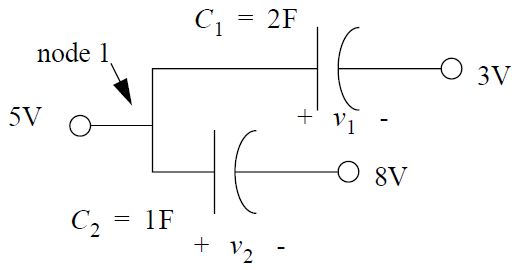
The charge on node 1 is found as follows:

Multiterminal Capacitors: Maxwell Capacitance Matrix

The Maxwell capacitance matrix is an electromagnetics concept that assists in dealing with interactions between many different conductors. Say there are three different conductors, each at its own voltage. The charge on conductor 1 is partly determined by its own voltage and partly by the voltages on the other two. The relationship is linear:

Similar relationships hold for conductors 2 and 3. The role of a field solver is to compute the various coefficients , where indicates the charge induced on conductor by a 1 volt voltage on conductor . In linear, isotropic dielectric materials, these coefficients are reciprocal; that is, .

The collection of these capacitance coefficients is known as the Maxwell capacitance matrix . For the 3-conductor example, the Maxwell capacitance matrix could be written as:

This employs the reciprocity condition to replace with , etc. This is the capacitance matrix that the field solvers in Q3D Extractor compute.

Spice Capacitance Matrix

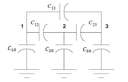
The figure below shows a set of two-terminal capacitors connected between ground and three other nodes (1, 2, 3).

Assume that the voltages and on nodes 1, 2, and 3 are known.  The total charge on these nodes can be computed.  For example, on node 1 the total charge is:

Therefore, there is a relationship between the two-terminal capacitor values and the entries of the Maxwell capacitance matrix:

And so on.  The diagonal entries of the Maxwell capacitance matrix are found by summing the total of all two-terminal capacitances connected to the given node. The off-diagonal entries of the Maxwell capacitance matrix are found by taking the negative of the coupling capacitance between two nodes.

Thus, the Maxwell capacitance matrix is given in terms of two-terminal capacitor values as:

An alternative representation of the Maxwell capacitance matrix, known as the Spice Capacitance Matrix, is available in Q3D Extractor.  The Spice Capacitance Matrix collects the values of the two-terminal capacitors that would give rise to the same charge relationships that the Maxwell capacitance matrix describes. 

For the example above, the Spice Capacitance Matrix is:

The diagonal entries of the Spice capacitance matrix are the sum of the rows of the Maxwell capacitance matrix:  .  The off-diagonal entries of the Spice capacitance matrix are the negative of the corresponding entries of the Maxwell capacitance matrix:  for .

Multithermal Capacitors in Lossy Dielectrics: Conductance (G) Matrix

When Q3D Extractor solves a problem involving lossy dielectric materials, the losses give rise to a non-zero conductance (G) matrix. The G matrix can be visualized as a set of two-terminal resistors connected in parallel with each of the two-terminal capacitors in this figure:

These resistors are characterized in terms of their conductance values (the reciprocal of their resistance), measured in siemens.

The G matrix relates the leakage currents in the dielectrics to the conductor voltages. Thus, a system of two conductors gives a 2x2 conductance matrix:

The leakage currents are then given by:

Admittance (Y) Matrix

In many cases, when Q3D Extractor performs matrix reduction operations, the capacitance matrix and the conductance matrix are affected in the same way.  In these cases, the same reduction formulas apply to both the G and C matrices.  However, for certain operations these matrices must be combined to work in terms of the admittance (Y) matrix. The entries of the Y matrix are where is the angular frequency. 

The admittance matrix must be used when a problem requires Q3D Extractor to enforce conditions on the total current. For example, when floating a conductor in a lossy problem, its total current must equal zero.

The matrix reduction operations that require use of the admittance matrix are: floating a conductor and floating at infinity. 

To simplify the information that follows, these operations are explained in terms of the capacitance matrix, as if the problem were lossless. The results derived could also apply to a lossy problem if were replaced by   The reduced Y matrix can be separated into the reduced G and C matrices by taking the real and imaginary parts, respectively, and then dividing the imaginary part by to obtain C.

Two-Terminal Inductor

The figure below shows an ideal two-terminal inductor with its branch voltage, branch current, and magnetic flux.

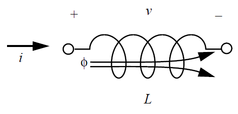
A two-terminal inductor is described by the following relationship between its branch voltage and the time derivative of its branch current :

It’s often convenient to instead separate this into two separate relationships. The magnetic flux is defined as:

Accompanying this is the relationship between voltage and the time derivative of the flux:

For this example, force the voltages on two inductors to be equal to one another; in other words, , or:

Assuming there was some time in the past when both inductances were completely discharged, integrate this equation to arrive at the result:

It is often more convenient to work with inductor fluxes than voltages, as this avoids carrying the time derivative operator.

Coupled Inductances

Two coupled inductances have their fluxes determined by the currents in both inductors:

The quantities are the entries of the inductance matrix for these two conductors:

The voltages across these coupled elements are computed from the fluxes in exactly the same way as for uncoupled elements:

It is easy to expand these two relationships in terms of time-derivatives of the two currents. It is also straightforward to generalize from the case of two coupled inductances to an arbitrary number of couplings.

Resistance and Mutual Resistance

The relationship that describes a two-terminal resistor is the familiar Ohm’s law, which relates branch voltage to branch current :

In certain situations, it is meaningful to consider mutual resistance effects. The simplest case to visualize is the multiterminal conductor (“net”) shown below.

This figure demonstrates mutual resistance between two current-carrying paths on the same multiterminal conductor. In this example, a current flowing into one terminal produces voltage drops throughout the conductor. Part of this voltage drop is across the bottom leg of the Y shape. This portion of the voltage drop is shared between and , and so it appears in both. The "shared" voltage drop creates mutual resistance. Consider:

Thus, the mutual resistance is the voltage drop sensed by due to a one ampere current flowing in . For linear, isotropic media, this is the same as the voltage drop induced in by a 1 amp current in .

When dealing with multiple conductors, it is natural to describe them with a resistance matrix. For the two-conductor example, the resistance matrix would consist of the self-resistances on the main diagonal and the mutual resistance values between the conductors on the off-diagonals:

Impedance (Z) Matrix

The resistance matrix and inductance matrix usually behave in the same way when the matrix reduction operations in Q3D Extractor are applied. The same formulas that yield the reduced L matrix will yield the reduced R matrix. However, for certain operations, the resistance and inductance matrices must be combined to work in terms of the impedance (Z) matrix.  The entries of the impedance matrix are where is the angular frequency. 

At non-zero frequency, the voltage on a conductor will have resistive and inductive components. Therefore, the impedance matrix must be used when the matrix reduction operation enforces conditions on the voltage drop.  These cases include:  joining conductors in parallel, joining selected terminals, and grounding a conductor.  For simplicity, the reduction formulas for these operations are derived as if the problem were lossless (having zero resistance). 

The results obtained will also apply to problems with non-zero resistance if is replaced by the impedance in the formulas.  As with the admittance matrix, the reduced impedance matrix, once computed, can be separated into the reduced R and L matrices by taking the real and imaginary parts of Z respectively and then dividing the imaginary part by to get L.