
Creating a Fields Report
The following is the general procedure for creating any type of Fields Report. It includes drawing a polyline to use as the path along which thermal results will be plotted or tabulated. This step is necessary for the predefined temperature, heat flux, and loss results. However, you can plot or tabulate Design Volumes and Named Expressions you create using the Fields Calculator (see note below) without creating any polyline geometry.
The Fields Calculator is a powerful and flexible tool for post processing your analysis results. Use it to perform simple or complex mathematical operations on the raw results data. With an appropriate named expression defined, you can generate a report that does not require a polyline as its basis. For example, you could define a face list and create a named expression that integrates the heat flow rate for all faces in the list. Then, in a parametric analysis, you could base the plot's X axis on a design parameter. Finally, base the plot's Y axis on your named expression, thus creating a plot of total heat flow rate of the faces versus the swept parameter. There are many other possibilities as well.
You can access the Fields Calculator by right-clicking Field Overlays in the Project Manager and selecting Calculator from the shortcut menu. For more information, search the Ansys Electronics Desktop help for "using the fields calculator" (include the quotation marks to limit search results to instances of the full phrase). Also, refer to the Related Topics links at the bottom of the Using the Fields Calculator page.
- Optionally, if you will be plotting thermal results in the spatial domain, create a polyline path to use as the basis of the table's or plot's X data using one of the following two methods:
- Draw a polyline manually:
- On the Draw ribbon tab, click
 Draw line.
 - If prompted to create a non-model object (because a solution already exists), click Yes.
- Draw a line or series of lines along which you wish to determine the thermal results. The line segments should pass through or along the surfaces of the bodies comprising the model. Use one of the following three drawing methods:
- Specify the line start and end points graphically (by clicking in the Modeler window). You can snap to model vertices (endpoints), midpoints or edges, grid points, and more.
- Specify the points by typing the coordinates into the X, Y, and Z text boxes in the status bar.
- Draw an arbitrary line and edit it's properties afterward (in the docked Properties window or the Properties dialog box).
- After clicking the last endpoint, right-click in the Modeler window and choose Done to terminate the Draw Line command.
- Continue to step 3.
- Convert model edges to a polyline:
- In Edge selection mode, select a model edge or a contiguous series of model edges to select them.
- On the Draw ribbon tab, click
 Edge > Create Object From Edge.
 - While the objects are still selected, click
 Unite on the Draw ribbon tab.
 - Continue to step 3.
- Optionally, if you will be plotting thermal results in the time domain (transient solutions only), create a point to use as the basis of the table's or plot's Y data, as follows:
- On the Draw ribbon tab, click
 Draw Point.
 - Click a suitable grid point or snap point on the model (such as the midpoint of an edge, quadrant point on a circular edge, center of a face, or vertex) to place a point there.
- Access the Report dialog box using one of the following three methods:
- On the Results ribbon tab, click
 Fields Report and choose the desired display type (such as,
  2D,
2D,  Data Table, or
  Stacked).
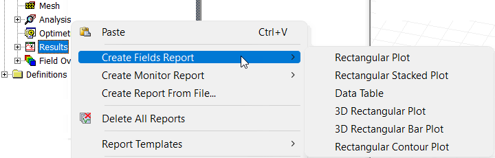
 - Using the menu bar, click Mechanical > Results > Create Fields Report > desired display type.
- Right-click Results in the Project Manager and choose Create Fields Report > desired display type:
- Specify the following settings in the Report dialog box:
- Choose the desired solution setup from the Solution drop-down menu (if you solved more than one setup).
- Choose the polyline or point you created previously from the Geometry drop-down menu.
- Optionally, for a polyline, specify a different number of Points to calculate along the specified polyline. (The default number of points is 101, which results in one hundred trace segments between the first and last data points.)
- In the Category list, select Calculator Expressions, if it is not already selected.
- Select the desired Quantity or Quantities to tabulate or plot. (You do not need to specify a Function for thermal results.)
- Optionally, click Range Function to apply a mathematical operation to the results. Then:
- In the Set Range Function dialog box, choose the desired operation from the Function drop-down menu (such as sum, mean, max or variance).
- Click OK to return to the Report dialog box.
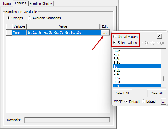
- Optionally, if there are multiple design variants (such as in a Parametric analysis) or multiple time steps (in a transient solution), click the Families tab to choose the ones to plot. Then:
- Click the ellipsis button in the Edit column:
- Choose Use all values or choose Select values and pick individual values to include in the plot.
- Click New Report.
- Optionally, if you created a plot, you can double-click inside the legend box to access the Properties dialog box and customize many plot parameters, such as:
- Trace colors, style, and width
- Enable data point symbols and change their color, fill, style, and frequency
- Grid options
- Headers
- X and Y axis parameters and scaling
- Optionally, if you created a data table, you can customize it in the following ways:
- Drag the column borders to resize the columns.
- Click on a column heading and then, in the docked Properties window, adjust the Units, Field Width, or Field Precision values.
- Optionally, select parameters for one or more additional results to add to the current plot or table and click Add Trace.
- Click Close to exit the Report dialog box.
You can switch between straight and curved segments by right-clicking in the Modeler window and choosing the desired Set Edge Type option.
Notice the name of the line object that has been added to the History Tree. The default name for the first line object is Polyline1, and you can change the name in the docked Properties window if desired.
Notice the name of the united object that has been added to the History Tree. You can change the name in the docked Properties window if desired.
Alternatively, tab into the coordinate entry text boxes at the bottom of the program window, type the exact coordinates of the desired point, and press Enter.
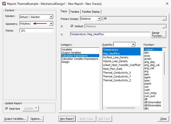
The following report setup example shows the settings to tabulate or plot Temperature and Mag_HeatFlux results along Polyline1:
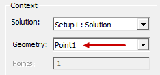
To tabulate or plot Temperature and Mag_HeatFlux at a point versus Time (transient solutions only), the setup would be the same as the preceding example, except for the Geometry selection:
You can also choose polyline geometry for plotting the results of a transient solution. However, the plot with be in the spatial domain, with the distance along the polyline as the X axis. A separate curve will be added to the plot for every time value selected under the Families tab.
The plot or data table appears in a new window.
Examples:
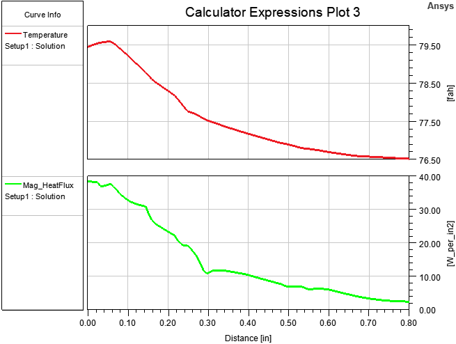
The following example is a stacked rectangular plot of the Temperature and Mag_HeatFlux results along Polyline1. The polyline was drawn from the center of a transistor/heat sink contact face to one of the bottom corners of the heat sink. The temperature and heat flux decrease with increased distance from the heat source:
The following example is a data table listing the volume of the three objects comprising a model. It has been modified to show the volumes in cubic inches, and the columns have been reduced from their default widths:
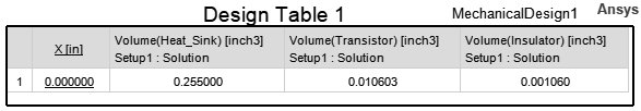
The contents of the Y text box in the Report dialog box used to produce the preceding table were as follows:

In this example, an additional column has been added to Design Table 1:
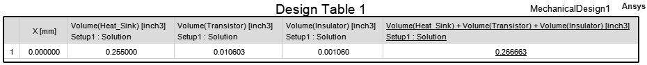
With the Volume of all three parts selected in the Quantity list of the Report dialog box, the semicolons in the Y text box were replaced with plus signs (+):

to produce the total volume column (far right).