
Mathematical Method Used in HFSS
The numerical technique used in HFSS™ is the Finite Element Method (FEM). In this method a structure is subdivided into many small subsections called finite elements. In HFSS these finite elements are in the form of tetrahedra. The entire collection of tetrahedra constitutes the finite element mesh. A solution is found for the fields within these tetrahedra. These fields are interrelated so that Maxwell’s Equations are satisfied across inter-element boundaries yielding a field solution for the entire original structure. Once the field solution is found, the generalized S-matrix solution is determined. The following figure shows the geometry, mesh, field results, and the S-matrix results of a bandpass cavity filter in HFSS.
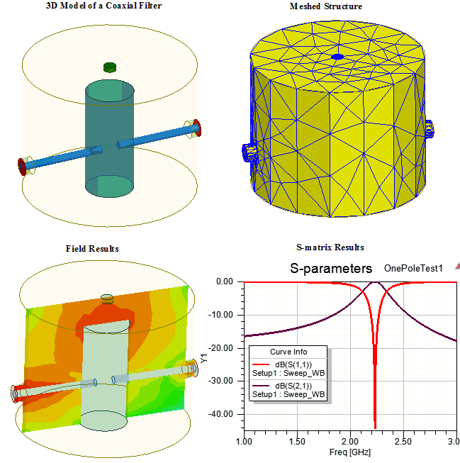
A sample HFSS model with mesh plot and results
Subject to excitation and boundary conditions, HFSS solves for the electric field E using the following equation:

where

 are the relative
permittivity and permeability respectively and c is the speed of light
in vacuum.
are the relative
permittivity and permeability respectively and c is the speed of light
in vacuum.
Note  is used to represent any source.
HFSS calculates the magnetic field H using the following equation:

The remaining electromagnetic quantities are derived using the constitutive relations.
From the quantities used in equations (1) and (2) it’s clear that a problem in HFSS is considered in terms of electric and magnetic fields rather than in terms of voltages and currents. Consequently, it is important that an HFSS simulation includes a volume within which electric and magnetic fields exist. These volumes generally comprise of dielectrics and conductors (including air, that surround the conductors).
HFSS derives a finite element matrix using the field equations to calculate the fields and S-matrix associated with a structure excited with ports.
The procedure to solve the problem in HFSS can be briefly described as follows:
- A geometric structure is represented by a finite element mesh using tetrahedral elements.
- Testing functions Wn are defined for each tetrahedron, resulting in thousands of basis functions.
- The field equation is multiplied by Wn and integrated over the solution volume
This procedure yields thousands of equations for n=1,2,…,N.

After manipulating these N equations and using Green’s theorem and the divergence theorem the following equation is obtained:

for n=1,2,…,N writing,

rewrites (3a) as,

for n=1,2,…,N
Equation (5) then has the form

or

In this matrix equation, A is a known NxN matrix that includes any applied boundary condition terms, while b contains the port excitations, voltage and current sources and incident waves.
E can be calculated when equation (7) is solved for x.
In HFSS the shape functions or testing functions Wn (appearing in the above equations) are vectors. They are curl conform which essentially means that the tangential continuity of the E field is maintained. They are also hierarchical with variable polynomial order. In other words the higher order polynomial shape functions are appended to the lower order polynomial shape functions. Different orders of basis functions employ different interpolation schemes for interpolating field values from the nodal values. This property is imperative for the iterative solver.
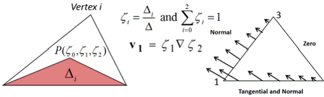
Hierarchical vector basis functions
The field solution process utilized by HFSS is iterative. In other words, HFSS uses the above process repeatedly by refining the mesh in an intelligent manner, until the correct field solution is found. This repetitive process is known as the adaptive mesh refinement process that yields highly accurate results.
For example, consider a simple waveguide structure. Initially, HFSS computes the modes on the cross-section of the waveguide. These modes serve as port excitations for the waveguide. HFSS uses a two dimensional FEM solver to calculate these modes. This initial calculation is referred to as the “port solution.” Once the port modes are known, they are used to specify the b matrix.
After the right hand side of equation 7 is determined, HFSS computes the full three-dimensional electromagnetic fields within the solution volume using the adaptive solution process. When the final fields are calculated, HFSS derives the generalized S- matrix for the entire model.
Note: The gamma results and characteristic wave impedance Zo that HFSS displays in a matrix data for a given simulation are essentially the transmission line properties of the modes of the wave port.