HFSS Multipaction Analysis

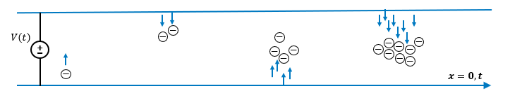
HFSS Multipaction provides a finite element approach to simulating vacuum multipaction in space-born communications systems and vacuum electron devices. When space charges are accelerated by time-harmonic fields in a confined space surrounded by materials, the charges can knock electrons off the material surfaces. If the transit time is in sync with the time-harmonic fields, the electron multiplication can be sustained and will eventually lead to an electron avalanche.

Detecting multipaction through measurement is difficult and expensive for a large antenna feed network on a satellite. Failure is also not an option for a mission-critical space project. Therefore, there is a big incentive to run computer simulation for identifying components prone to multipaction before launching a satellite into space. HFSS can guide the design of multipaction suppression measures.

HFSS Multipaction supports multipaction on both metallic and dielectric surfaces. You can set up a uniform DC bias field as part of HFSS Multipaction, or use Maxwell near field links to set up non-uniform DC bias fields. This is helpful in design and simulation because multipaction is less likely to happen after applying magnetic bias.

Optionally, you can select the Charge distribution option in the Multipaction Analysis setup to output particle and geometry mesh information used to produce particle plots and animations.

Prerequisites

• A multipaction analysis requires the time-harmonic fields being saved for a driven-terminal or driven-modal solution.
• While HFSS Multipaction can simulate uniform bias, to simulate the effect of non-uniform bias fields, use Maxwell near-field links.

General Multipaction Analysis Process

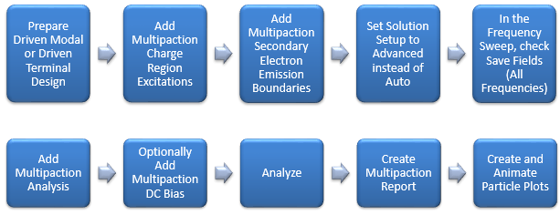
The process flow for running Multipaction Analysis follows:

If you want to creation particle animations, you must select the Charge distribution option in the Multipaction Analysis setup to output particle and geometry mesh information.

Prepare a Driven Modal or Driven Terminal Design

As stated above, a multipaction analysis requires the time-harmonic fields being saved for a driven-terminal or driven-modal solution. Therefore, the multipaction setup and associated boundary conditions apply only to these types of HFSS projects. Other solution types, such as transient, eigenmode, characteristic mode, and SBR+, do not support the multipaction analysis. In addition, a multipaction simulation currently does not support renormalization or deembedding of ports.

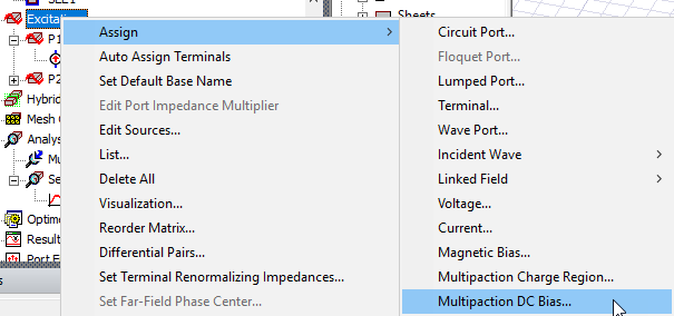
Add Multipaction Charge Region Excitations

In HFSS Multipaction, charges are added to the simulation domain as excitations. A Multipaction Charge Region consists of either multiple objects or multiple faces, depending on whether the Selection Mode is Objects or Faces.

This opens the Multipaction Charge Region dialog box.

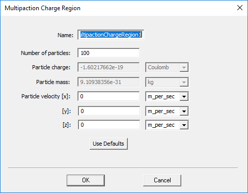
For each charge region, we can specify the number of electrons and their initial velocities. It is not necessary to seed charges in the entire simulation domain if the regions prone to multipaction can be easily identified, such as small gaps, coaxial feeds, parallel plates, and regions with strong fields. The simulation time can be significantly reduced by seeding charges only in critical regions.

The statistical variation of multipaction simulation can be reduced by using more particles, but the simulation time will increase as well. Moreover, using too few particles (less than 1000 for all charge regions) will introduce noises to the results and may trigger an early termination of the simulation.

Adding Multipaction Secondary Electron Emission (SEE) Boundaries

The Multipaction SEE boundaries should be added to vacuum-material interfaces where secondary electrons will be generated. Typically, those interfaces are associated with PEC, impedance, or finite-conductivity boundaries in electromagnetic simulation. If a Solve Inside object contacts the vacuum region, you should add SEE boundaries on their interface to avoid charged particles penetrating the object.

Charged particles will be entirely absorbed by surfaces in contact with vacuum but not covered by SEE boundaries. For example, port faces should not be covered by SEE boundaries because charged particles should be allowed to leave the simulation domain through ports.

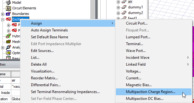
Select the faces or objects to which you want to assign SEE boundaries, right-click on Boundaries in the Project Manager, and select Assign> Multipaction SEE... This command opens the Multipaction SEE dialog box:

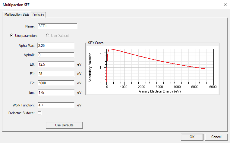
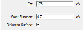
The secondary emission yield (SEY) depends on the impacting energy of the primary electron. We adopt an enhanced Vaughan model where the SEY curve will fall exactly on the low and high cutoff energies E1 and E2, where SEY is equal to 1. SEY reaches the maximum Alpha_Max for an energy Em in between E1 and E2. For low-energy primary electrons, SEY is equal to Alpha₀ when the impacting energy is between 0 and E0. The work function is needed for calculating the energy of secondary electron emission by the Chung-Everhart distribution. All energies related to the SEE boundary are measured in electron volts (eV). You must check the Dielectric Surface checkbox for an insulator-vacuum interface, which allows the accumulation of positive surface charges after secondary electrons leave the interface, or the accumulation of negative surface charges after the interface absorbs primary electrons.

Adding a Multipaction Setup

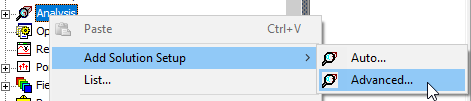
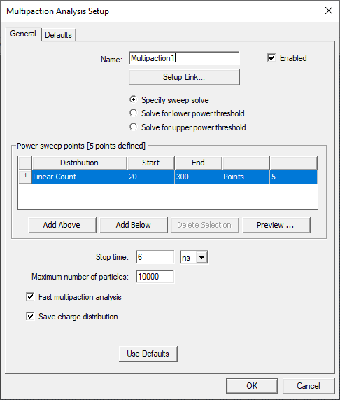
At least one charge region and one SEE boundary must exist before you can add a Multipaction Analysis. To add a Multipaction Analysis, you must add a Solution Setup and a Frequency Sweep. You then add the Multipaction Setup to the Sweep. When you add the Solution Setup to an Analysis in HFSS, select Advanced instead of Auto.

The frequencies specified in the frequency sweep will be reused for setting up the multicarrier signal for a multipaction analysis. You must select the Save Fields (All Frequencies) checkbox while editing the frequency sweep, otherwise Add Multipaction Analysis will be grayed out on the menu. There will be no multipaction if there is no time-harmonic field to sway the charged particles in the simulation domain.

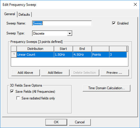
Once the above procedures are completed, you can right-click the frequency sweep and select Add Multipaction Analysis...

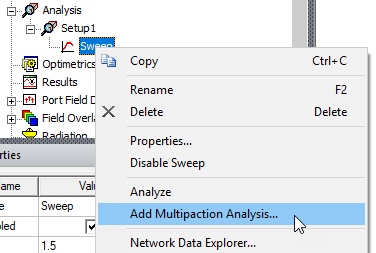
This opens the Multipaction Analysis Setup dialog box.

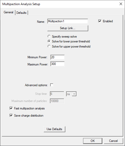
The Solve for lower power threshold button allows automatic determination of the lower power threshold. It is the power threshold where the breakdown status transits from no multipaction to multipaction with increasing input power. Similarly, the Solve for upper power threshold button allows automatic determination of the upper power threshold. It is the power threshold where the breakdown status transits from multipaction to no multipaction with increasing input power.

Given the power range provided by the user, the software determines which power multiplier to simulate next based on previous multipaction history, instead of reading preset power multipliers from a table. By default, the advanced options are off. The lowest power threshold is found using a stop time ranging from 80 to 120 RF cycles and no more than twice the initial number of particles. The default settings can be overridden by checking advanced options if users prefer to set up the parameters by themselves

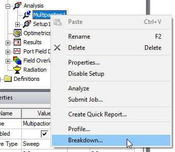
While the automatic simulation is running, you can check the breakdown status of simulated power multipliers by clicking Breakdown... under the multipaction setup shortcut menu.

This opens a Solutions dialog box with a Multipaction tab that provides Power and Breakdown information as follows:

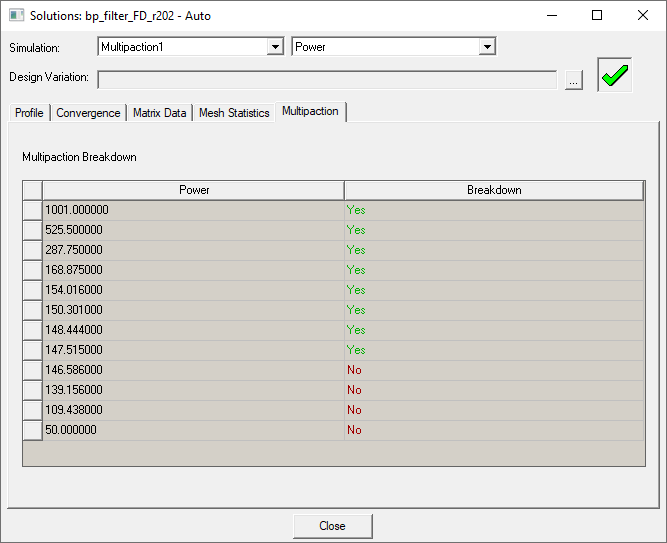
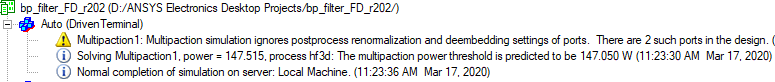
When the Auto Solve converges, there will be a message showing the lowest multipaction power threshold in the Message Manager window.

If the Auto Solve does not converge, it means the structure is free of multipaction for given geometry, material, and simulation setups.

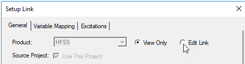
Whether you choose Sweep Solve or Automatic Solve, you have to click Setup Link… to link the multipaction analysis with a frequency sweep before running the multipaction simulation.

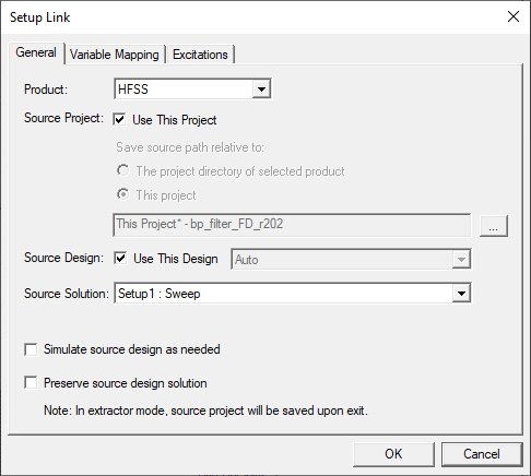
By default, the link points to the current project, design, and sweep. After setting up the source, click the Excitations tab so you can specify the excitations or the DC bias fields for the multipaction analysis.

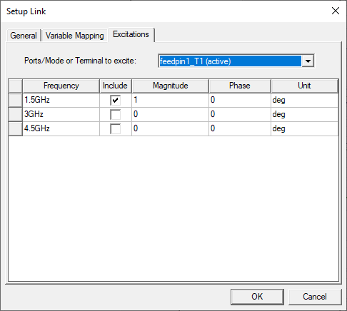
You must include at least one terminal with a positive magnitude. The input signal for each mode or terminal is a linear combination of multi-carrier signals multiplied by the square root of the power multiplier:

where is the port voltage of the i-th carrier with one-watt input power in driven-modal solutions. For driven-terminal solutions, the input power of a port is not one-watt. Therefore, scaling must be done before applying the above formulation for calculating the port voltage.

After setting up the excitations, press OK to complete the link setup. Afterward, you can only edit the Setup Link if you click Edit Link. Otherwise, the Setup Link dialog box will be in read-only mode.

The second step in the Multipaction Analysis dialog box, if you have selected Sweep solve, is to set up the stop criteria by a stop time and the maximum number of particles.

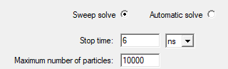
The multipaction simulation will be terminated according to the stop time, which is usually set to 20 cycles of the lowest frequency of the multicarrier signal. The simulation also terminates when the number of particles reaches zero or exceeds the maximum number of particles.

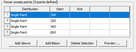
The third step for Sweep solve is to specify power sweep points or multipliers for scaling the power of each port mode or terminal voltage. Each mode in a driven-modal design, or each terminal in a driven-terminal design has one-watt input power. When there is only one mode or one terminal active, the power multiplier is essentially the input power of the multipaction analysis.

The fourth step for both Sweep solve and Automatic solve is to select whether the multipaction analysis type will be fast or not. The fast simulation is less compute-intensive but also less accurate when the structure to be analyzed has complex geometry and fine details. However, our tests show that the fast simulation is satisfactory for most applications.

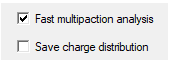
The last step is to choose whether to write out Charge distribution and model geometry. This data can be displayed as particle overlays and animations in Electronics Desktop.

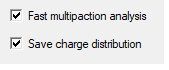
Saving charge distribution involves writing to a hard drive and will slow down the simulation. If the goal is to predict the multipaction power threshold, the overhead can be avoided by unchecking the option.

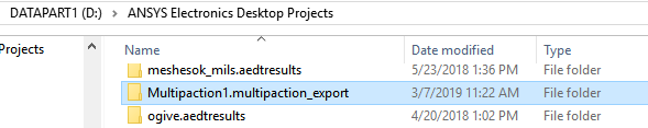
The model and particle files (*.vtu) will be written to a directory at the same level as the HFSS project:

Optional Multipaction DC Bias

It is optional to set up DC electric or magnetic bias fields for a multipaction analysis.

This opens the Multipaction DC Bias dialog box.

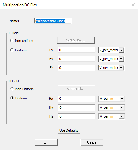
The type of bias can be either uniform or nonuniform. For a uniform bias, the field values are the same throughout the entire simulation domain. The non-uniform bias fields are specified through Maxwell near field links.

Running the Multipaction Simulation

Once the multipaction setup is completed, right-click the multipaction analysis and select Analyze to run the multipaction simulation.

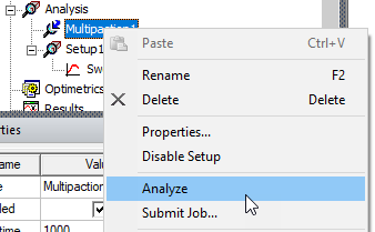
If the 3D field solutions of the linked frequency sweep and the Maxwell projects are not available, additional HFSS and Maxwell simulations will be invoked as shown in the Progress window.

Plotting the Charge Evolution

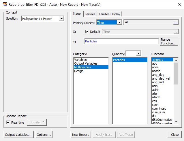
The final step is to plot the charge evolution through multipaction plots. You can right-click on results, select Create Multipaction Report, and select the report type.

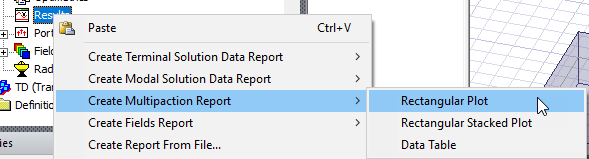
You can also access the Multipaction Reports on the Results tab of the ribbon.

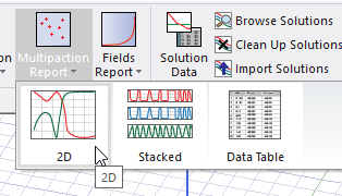
In the Report dialog box, select Multipaction as the Category and Particles as the Quantity.

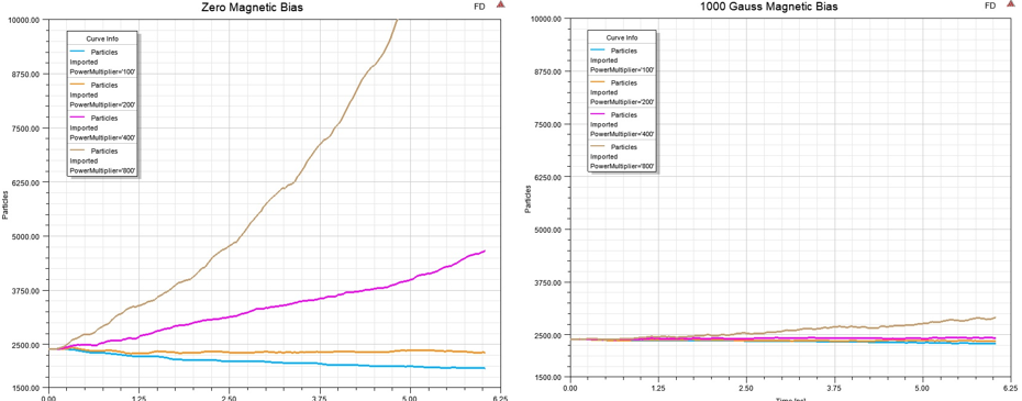
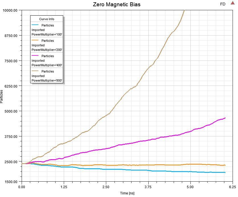
The following example report shows the results with different PowerMultipliers and Zero Magnetic Bias.

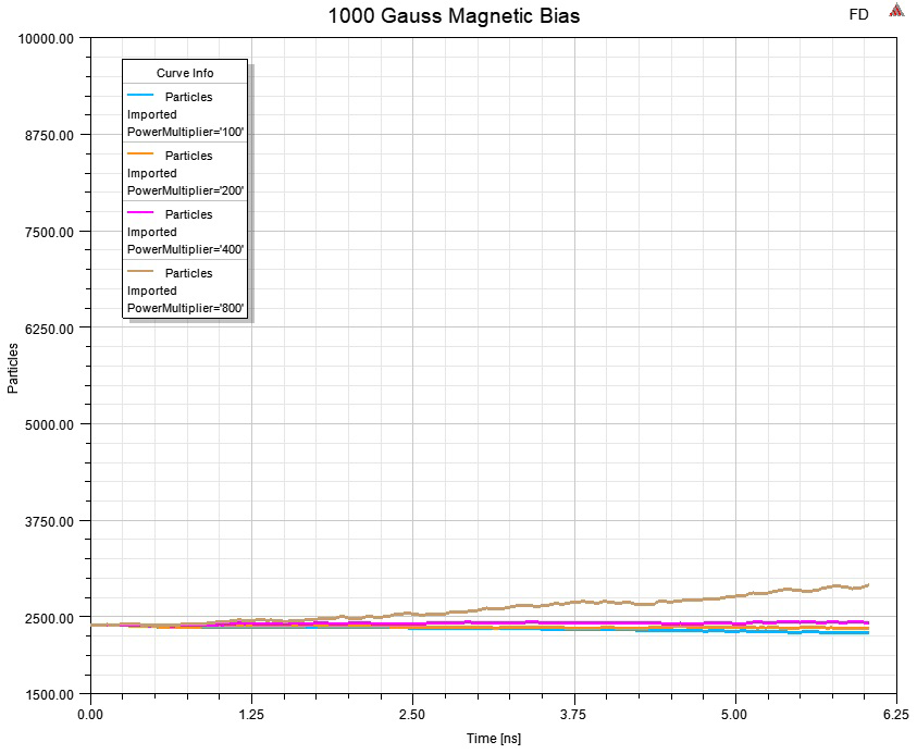
The following example shows a range of power multipliers with a 1000 Gauss Magnetic Bias assigned.

Displaying and Saving Charged Particle Animations

In order to display a charge particle animation, you have to select Charge Distribution in the Multipaction Analysis Setup dialog box.

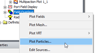
Once the multipaction simulation is finished, you can right-click Field Overlays and select Plot Particles....

This opens the Create Particles Plot dialog.

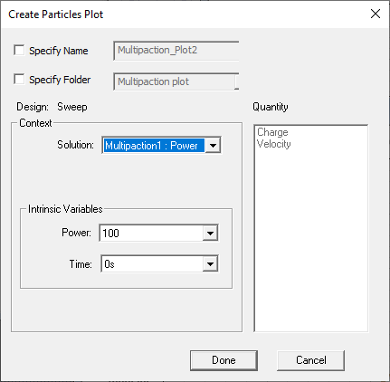
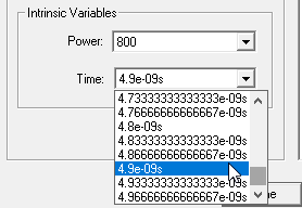
When there are multiple multipaction setups and power multipliers, the dialog allows you to select specific Solution and Power to plot the charged particle distribution and animation.

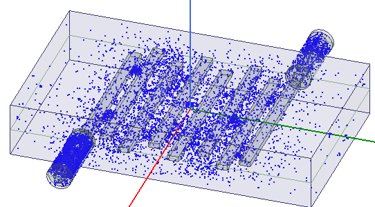
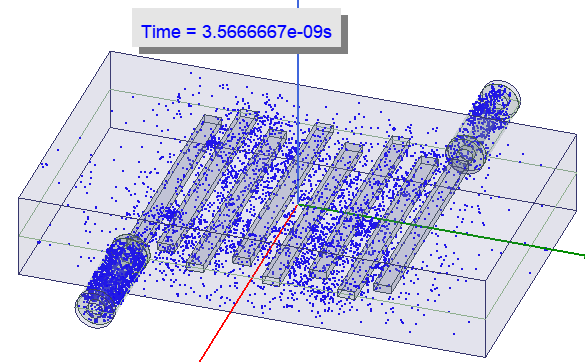
Click Done to cause a Particle plot to appear in the Modeler window.

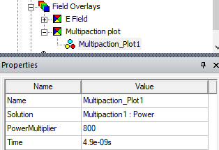
The properties of the particle plot are shown in the Properties window.

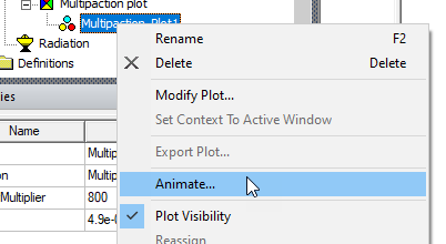
Once you have generated the Multipaction Plot in the Field Overlays, you can create an animation of the movement of the charged particles. Right-click the Multipaction Plot and select Animate... from the shortcut menu.

If you have previously created an animation for the plot, the Select Animation dialog box will open. You can select an animation to view, Edit, or Delete, or select New... to open the Create Animation Setup dialog box. If you have not previously created an animation, the Create Animation Setup dialog opens automatically.

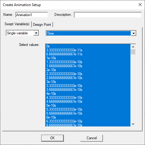
By default, the charge distribution for all time steps will be animated. The animation comes with a label showing the current time.

You can remove the label by unchecking Show in the Animation control panel.

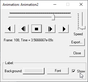
To save an animation file, click Export... and choose the path and file type of the animation.

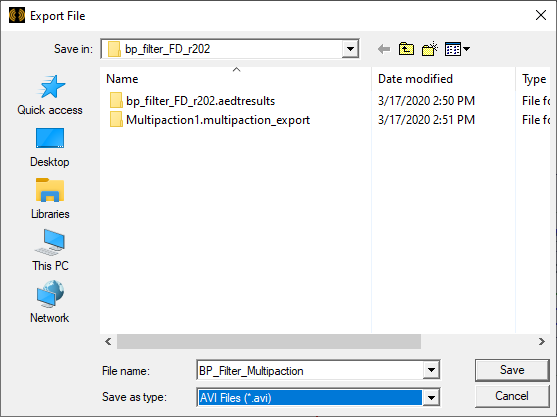
Files can be AVI Files (*.avi), Animated GIF (*.gif), or Web M Files (*.webm).

To Store and Obtain Power via a Script

You may want to get the power threshold for each autosolve analysis without reading the entire breakdown status table and figuring out the power threshold through a complicated script. You can access the power threshold through a single line of script. Although the power threshold should not be time-dependent, with the current implementation we can sample the value at t = 0.

# ----------------------------------------------

# Script Recorded by Ansys Electronics Desktop Version 2025.1.0

# 10:55:07 Jun 05, 2024

# ----------------------------------------------

import ScriptEnv

import ctypes

ScriptEnv.Initialize("Ansoft.ElectronicsDesktop")

oDesktop.RestoreWindow()

oProject = oDesktop.SetActiveProject("JPL_coax_power_threshold_r251")

oDesign = oProject.SetActiveDesign("Coaxial_7-8")

oModule = oDesign.GetModule("OutputVariable")

oModule.CreateOutputVariable("GetPowerThreshold", "PowerThreshold", "100MHz_low : Power", "Multipaction", [])

PowerThreshold = oModule.GetOutputVariableValue("GetPowerThreshold","Time='0","100MHz_low : Power", "Multipaction", [])

ctypes.windll.user32.MessageBoxW(0, str(PowerThreshold), "Power Threshold", 1)