Emission Test

The Emission Test in HFSS is intended for EMC analysis. EMC regulations specify the maximum radiated emissions as a function of frequency. The Emission Test in HFSS produces a plot that can be compared with these regulations. Assuming that the HFSS simulation contained a frequency sweep in which all the fields were saved (a fast frequency sweep is very suited for this), the Emission Test does the following:

1. It steps through the frequencies of your sweep;
2. At each frequency, it determines the maximum value of |E| on a sphere around the radiating device, regardless of direction;
3. It plots this |E_max| as a function of frequency. Optionally, |E_max| is scaled to account for the spectral density of a pseudo-random digital signal.

Geometry, S-parameters and antenna pattern

Let's start with a small model that solves quickly. Figure 1 shows an open-ended rectangular waveguide of which two side walls are perfect-H walls. Symmetry has been exploited twice, so we end up with a quarter of the geometry.

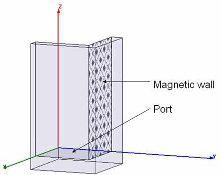
Fig. 1 The geometry: waveguide without cut-off

Around the waveguide is a larger volume of air with a radiation boundary. The model has been solved from DC to 12 GHz. Figure 2 shows the S parameters.

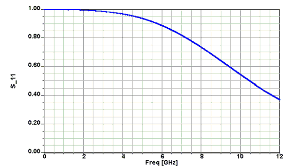
Fig. 2 S11 of the open-ended waveguide with two magnetic walls

Figure 3 shows a plot of the electric field at 12 GHz on a sphere with a radius of one meter. In this case, this is already way in the far field, so we are really dealing with radiated fields. Note that the electric field has a maximum of 28.8 V/m.

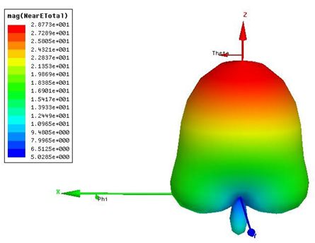
Fig. 3 Radiated electric field on a sphere with radius one meter

The average value in figure 3 is roughly 14 V/m. This corresponds to a power flux of 0.5|E×H| = 0.5|E|²/Z = 0.5×196/377 W/m² = 0.26 W/m². Over the sphere, area 4p m², this gives a power of 3.3 W. This value makes sense: the power into a quarter model is 1 W, so the total

power is 4 W, of which a small fraction is reflected back to the source.