Waveguide FEM versus Theory

Abstract

An example of solving a Rectangular and Circular Waveguide for the propagation constant, frequency cutoff, and wave impedance, by the finite element method (FEM), while making a detailed comparison to theoretical values derived from solving Maxwell's equation for metallic waveguides.

Simulation Time (adaptive solution, frequency sweep, and parametric sweep with 8 cores, 2025 R1):

Rectangular: 2 minutes:3 seconds Max. RAM per process = 201 MB)
Circular: 3 minutes:20 seconds (Max. RAM per process = 247 MB)

Note:

Simulation time and memory will vary depending on your available resources. In most cases, HPC (parallel resources) can be leveraged to significantly reduce simulation time and the memory footprint required by each CPU.

Model and Setup Details

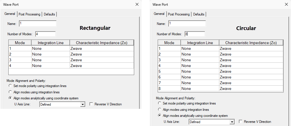
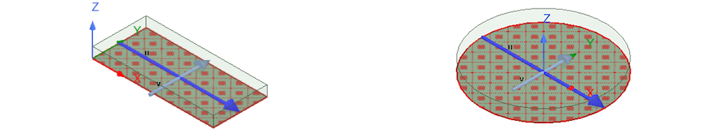
The models are drawn using the box or cylinder primitive, with parameters to control dimensions and solved as a single Ports Only solution, as we simply need the port properties for this study. Background PEC setting provides the metallic outer boundary, waveguide length is not relevant in this “ports only” example, so is set to a default 2mm. The model is set to solve with required number of modes, Characteristic Impedance Zo method is set to Zwave to give the wave impedance for comparison with theory. Mode alignment is set analytically as shown below.

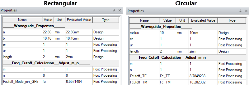
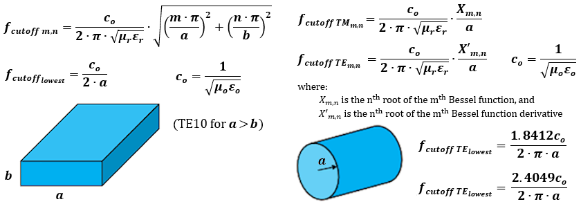
Wave port properties for the rectangular and circular waveguides

Wave port visualizations for the rectangular and circular waveguides

Model parameters are defined to scale the waveguide dimensions (a and b for rectangular, radius for circular). Additional parameters demonstrate how to evaluate the cutoff frequencies analytically using the TE/TM mode indices m and n, as per convention – design equations are shown below. These properties are postprocessing parameters and can be changed to check expected cutoff values for the guide dimensions and mode indices required. They are also used for mode identification in the mode table reports.

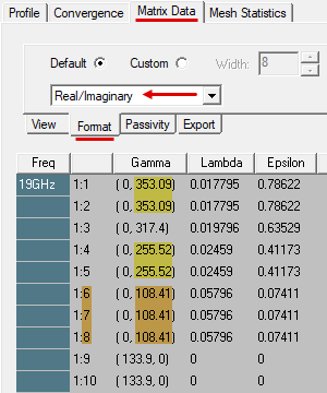
Design properties of the rectangular and circular waveguides

Cutoff frequency equations for the rectangular and circular waveguides

A single waveport is defined with the number of modes set as required. For this wideband test case, ensure that enough modes are enabled in the port setup to produce accurate results. Run the analysis initially with the frequency sweep disabled. Then, inspect the Matrix Data to evaluate the mode Gamma values with the Format set to Real/Imaginary. For example, with 10 modes set for the circular waveguide, we can see several modes have the same beta values (right/imaginary part of Gamma), indicating degenerate modes. So, if we wish to include mode 6, we should also include modes 7 and 8 (as shown in the preceding Wave Port dialog box image for the Circular design).

Matrix data showing real and imaginary gamma values for the circular design with ten modes specified.

The analysis setup and frequency sweep are defined based on the frequency span expected to evaluate the desired number of modes:

Rectangular:

Adaptive Frequency: 16 GHz
Sweep: 5–18 GHz in 10,001 points (1.3 MHz increments)

CylindricalWG:

Adaptive Frequency: 19 GHz
Sweep: 6–20 GHz in 20,001 points (0.7 MHz increments)

Initial mesh settings are adjusted only for the circular waveguide, with curvilinear elements enabled and a finer mesh slider position:

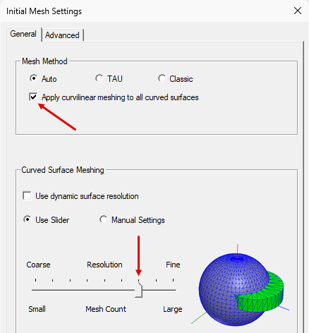
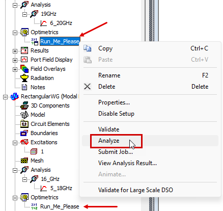
Initial mesh settings for the circular waveguide.

A Parametric sweep has been defined for each design to look at different combinations of the m and n indices (n^th root of m^th Bessel function and its derivative). Right-click and analyze each of these two parametric setups to run the adaptive solution, frequency sweep, and parametric sweep:

How to run all solutions from the Project Manager.

Postprocessing

Rectangular Waveguide:

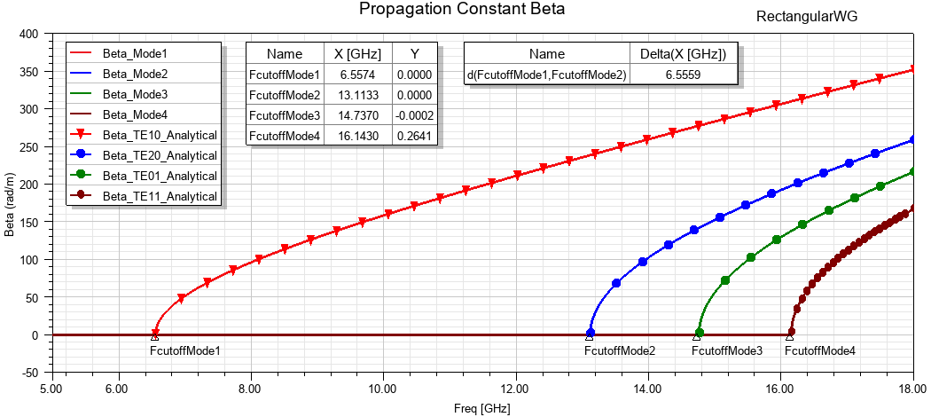
In the Project Manager, expand the Results folder in the RectangularWG branch to view the predefined reports. The Propagation Constant Beta plot shows the phase constant for the first four modes, with analytical calculations overlaid (defined as output variables). Trace markers (Add Minimum) are used to identify cutoff, a delta marker shows the single mode range (FcutoffMode1–2).

Propagation Constant Beta plot for the rectangular waveguide.

The TE/TM Mode table shows the evaluated cutoff frequencies for the modes as a function of indices m and n. You can use this table to confirm the FEM cutoff frequencies and to identify the modes.

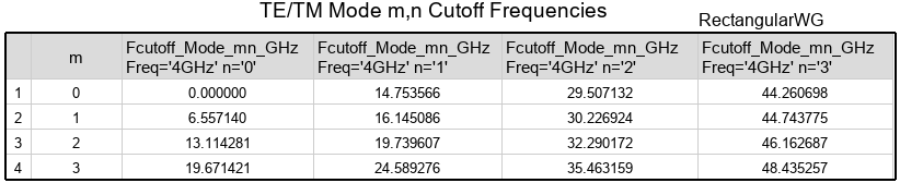
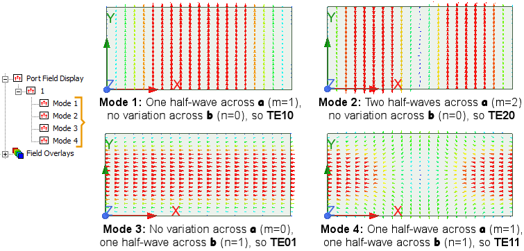
Mode TE slash TM, m by n Cutoff Frequencies table for the rectangular waveguide.

Mode 1: FcutoffMode1 (6.5574 GHz FEM / 6.5571 theory, 0.005% variance), can either be TE10 or TM01. The port field display (below) identifies it as TE10.
Mode 2: FcutoffMode2 (13.1133 GHz FEM / 13.1143 theory, 0.008% variance), can either be TE20 or TM02. The port field display identifies it as TE20.
Mode 3: FcutoffMode3 (14.7370 GHz FEM / 14.7536 theory, 0.113% variance), can either be TE01 or TM10. The port field display identifies it as TE01.
Mode 4: FcutoffMode4 (16.1430 GHz FEM / 16.1451 theory, 0.013% variance), can either be TE11 or TM11. The port field display identifies it as TE11.

You can make the final mode identification by using the Port Field Display for each mode:

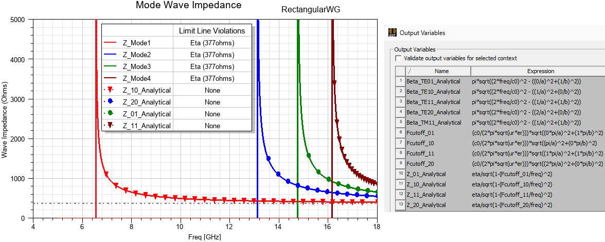
Port field displays for the four computed modes of the rectangular waveguide.

The Mode Wave Impedance plot shows the wave impedances (Zwave) compared to theoretical values defined using output variables:

Mode Wave Impedance plot for the rectangular waveguide.

Circular Waveguide:

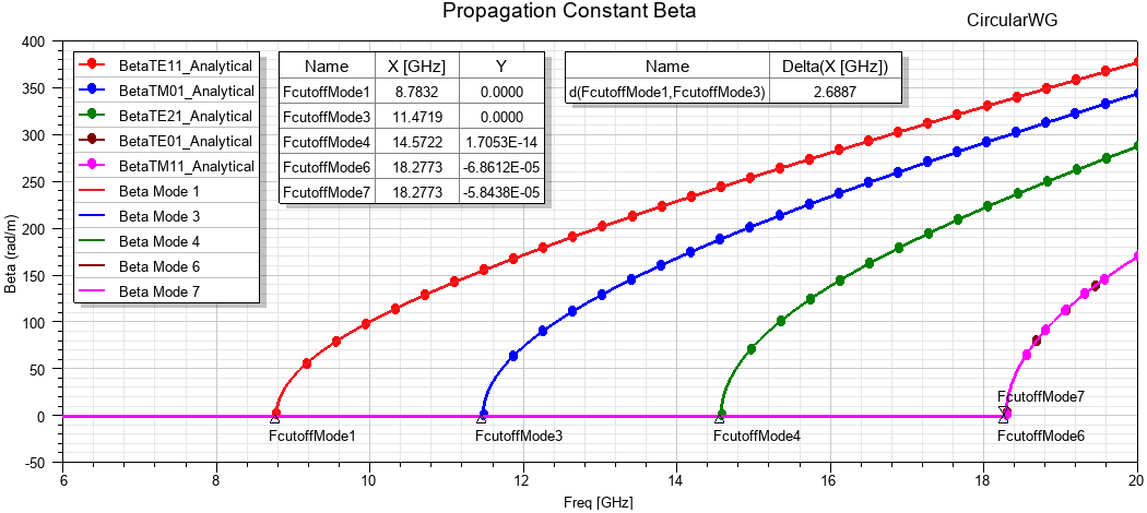
In the Project Manager, expand the Results folder in the CircularWG branch to view the predefined reports. The Propagation Constant Beta plot shows the phase constant for the first seven modes (ignoring degenerate modes 2 and 5), with analytical calculations overlaid (defined as output variables).

Trace markers (Add Minimum) are used to identify cutoff, and a delta marker shows the single mode range (FcutoffMode1–3) = 2.6887 GHz

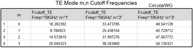
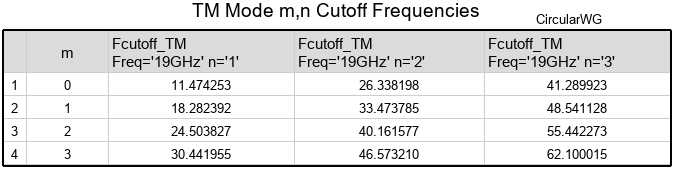
Propagation Constant Beta plot for the circular waveguide.

The TE Mode and TM Mode tables show the analytical cutoff frequencies for the modes as a function of indices m and n. You can use these tables to confirm the FEM cutoff frequencies and to identify the modes. Use the Port Field Display to confirm the following modes:

TE Modes table for all m and n indices showing Cutoff Frequencies for the circular waveguide

TM Modes table for all m and n indices showing Cutoff Frequencies for the circular waveguide

Modes 1, 3, and 4 are unique in the tables and easy to identify:

Mode 1: FcutoffMode1 (8.7832 GHz FEM / 8.7849 theory, 0.02% variance). From the TE Mode table, m=1 and n=1. Therefore, this mode is TE11.
Mode 3: FcutoffMode3 (11.4719 GHz FEM / 11.4743 theory, 0.02% variance). From the TM Mode table, m=0 and n=1. Therefore, this mode is TM01.
Mode 4: FcutoffMode4 (14.5722 GHz FEM / 14.5728 theory, 0.006% variance). From the TE Mode table, m=2 and n=1. Therefore, this mode is TE21.

Identify modes 6 through 8, for which the tables are inconclusive, using the Port Field Display:

Identifying Modes 6, 7, and 8 of the circular waveguide using the Port Field Display

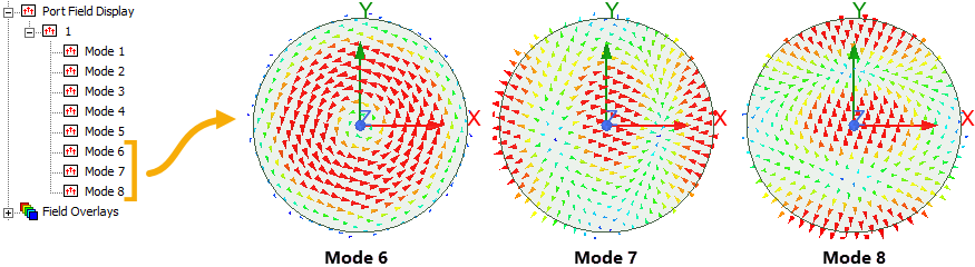
Mode 6: FcutoffMode6 (18.2773 GHz FEM / 18.2824 theory, 0.03% variance), this frequency appears in both mode tables, and it can be either TE01 or TM10. From the port field display, no field variation occurs around the circumference, so m=0. One minimum occurs along the radius, so n=1. Therefore, this mode must be mode TE01.
Mode 7 and Mode 8: (Same frequency as Mode 6) Two field maxima occur around the circumference, so m=1. One minimum occurs along the radius. Therefore, this mode must be TM11.

Note:

HFSS lists modes in order of decreasing Gamma value. For modes with the same Gamma value (for example, modes 6, 7, and 8), it is possible that HFSS may alter the order in which the modes are numbered due to numerical rounding.

The Mode Wave Impedance plot shows the wave impedances (Zwave) compared to theoretical values defined using output variables:

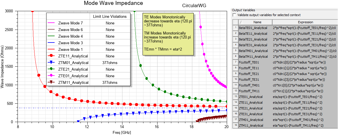
Mode Wave Impedance plot for the circular waveguide

Note:

In the preceding plot, the direction from which the Zwave curve approaches Eta (377 ohms) is helpful in determining whether the curve represents a TE or TM mode.

Interpolating Sweep Setup

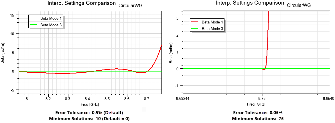
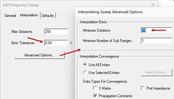
To accurately capture the abrupt change in Beta at cutoff, particularly when comparing it to analytical results, it may be necessary to adjust the interpolating sweep settings to improve fitting fidelity. Adjust these from the Edit Frequency Sweep dialog box (Interpolation tab).

Decrease the Error Tolerance (for example, 0.05%), click Advanced Options and increase Minimum Solutions (50–75) for better fitting at the zero point:

Adjusting the interpolating sweep's interpolation properties

A comparison of the results from the default and adjusted interpolation settings follows:

Comparison of the zero point accuracy resulting from the default and adjusted interpolation settings