Waveguide Combiner
Abstract
This HFSS example model is a rectangular waveguide combiner operating at 20 GHz.
This example project has an associated getting started guide:
- Getting Started with HFSS: 20 GHz Waveguide Combiner
Whereas the example model is fully set up, complete with predefined plots and overlays, and is ready to solve, the getting started guide offers an alternative learning path. Follow it to walk through the process of drawing the waveguide geometry, assigning the boundaries and excitations, setting up the analysis and frequency sweep, and postprocessing the results.
Solution Time: 4 cores in version 2025 R1 (meshing, adaptive solution, and frequency sweep)
Approximately 2 minutes, 255 MB max. RAM used
Simulation time and memory will vary depending on your available resources. In most cases, HPC (parallel resources) can be leveraged to significantly reduce simulation time and the memory footprint required by each CPU.
The WaveguideCombiner.aedt project file is located in the ...Examples\HFSS\RF Microwave subfolder of the program installation path.
Setup Description:
The waveguide combiner example has the following characteristics:
- E-plane symmetry boundary in the XY plane, so the model is half the height of the waveguide combiner it represents
- Impedance multiplier set to a value of 2 to account for the symmetry condition
- Wave ports assigned at each of the four inputs/outputs
- Finite conductivity boundary based on the properties of the material, aluminum, assigned to the bottom and the remaining side surfaces
- Analysis setup with an adaptive frequency of 20GHz, delta S = 0.005, and using second order basis (suitable for waveguide structures)
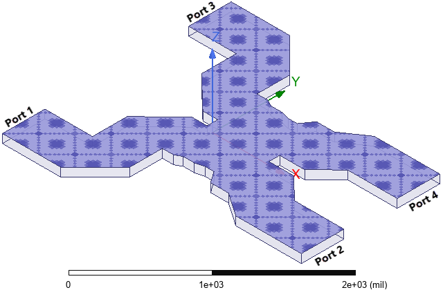
The following figure shows the waveguide combiner geometry with the symmetry boundary visualized:
Postprocessing
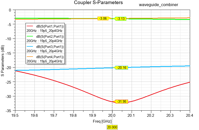
After analysis, the S-parameters can be seen in the predefined report, Coupler S-Parameters. X markers have been added to point out values at the 20 GHz adaptive solution frequency:
An E-Field overlay plot is also predefined to visualize the electric field distribution within the combiner. The field is controlled using the Edit Sources dialog box (to define the excitation magnitude and phase at each port). In this example, Port 2 is excited at 1 W of power and 0° phase. Port 4 is also excited at 1 W, but the phase angle is 90° (relative to the Port 2 phase). The remaining two ports are not excited (0 W):
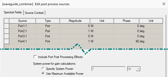
With the sources defined as shown above, the power from the two 1 W excitations will be combined, and essentially all of the output will be directed to Port 1:
The Phase annotation that appears in the Modeler window indicates the instantaneous phase of the excitation at Port 1 for each frame of the animation.
Optionally, change the Port 4 Phase value to various angles between -90° and 90°. You can Apply the port sources changes while the animation is running to immediately see the effect on the E-Field distribution (without closing the Edit Port Sources dialog box).
- With the Port 4 excitation at -90° phase, the input power is combined and essentially all of the output is directed to Port 3.
- At 0° phase, the outputs at Ports 1 and 3 are balanced.
- For Port 4 phase angles of -75° to -90° or 75° to 90°, the field strength will be very low at one of the output ports, and you can use a logarithmic scale to better see the weaker field color contours.
The following overlay animation shows the results with 1 W applied to both input ports and with a -60° phase angle at Port 4. In this case, the majority of the power is output at Port 3, with a lesser portion directed to Port 1:
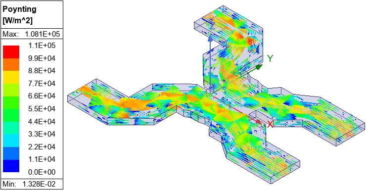
Streamline plots for vector quantities, such as Poynting Vector, can also be displayed. An example of the Poynting Vector is predefined and shown below. Select Poynting > RealPoynting1 under Field Overlays to visualize this result. Adjust the streamlines as desired by double-clicking the plot legend and adjusting the Seeds density in the Plots tab. This overlay shows the vectors with 1 W power and 0° phase at both input ports (2 and 4), in which case the output power is balanced between the two ports: