Twinaxial Cable

Twinaxial cables are used for in-rack connections between supercomputers to carry the networking traffic. They are meant for the transmission of short-range signals. The following figure illustrates a twinaxial cable (28 wire gauge) design, which comprises two inner conductors (S1 and S2) made of silver, and a shield or drain made of aluminum enclosed in an air-box. The central conductor is insulated with a dielectric layer.

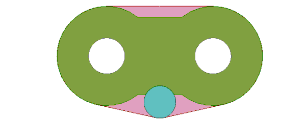
twinax cable design

The main intent is to draw a minimal length of the twinaxial cable and stretch it to any required length by using the post processing feature of Deembedding. Such a design saves simulation time and makes minimal use of computational resources and ensures efficient simulation, without explicitly modeling the actual length of the cable.

The design is parameterized as shown. The geometry is drawn using the parameters and boolean operations in such a way that all the individual objects that make up the geometry track with it. For example, when you change the values of the variables appearing in the Properties window, the model resizes accordingly and the objects with changed parameters are track with the geometry appropriately.

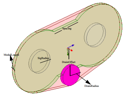
some of the parameters used in the design

Excitations

Right-click Excitations on the project tree and select List to open the Design List dialog box where you can select the terminals and wave ports that are assigned on this design. In the following figure, the two wave ports with their deembedding distances are highlighted.

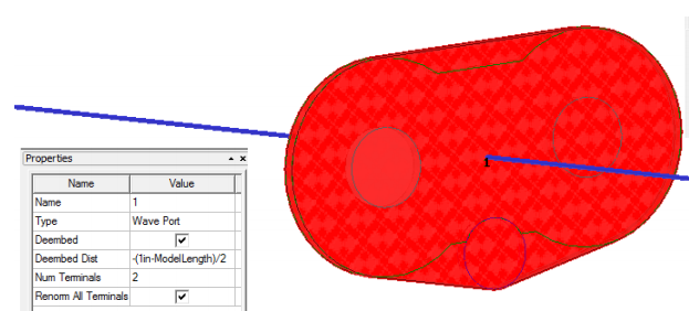
wave ports and deembedding

Negative values of deembedding indicates that the wave ports are deembedded away from the structure to stretch them to the required lengths. The transmission line characteristics are calculated along the shifted reference plane due to the deembedding. Deembedding prevents explicit drawing of the entire cable lengths. The following figure shows the 4 terminals assigned in this design.

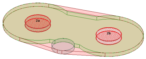
Twinaxial Cable terminals

HPC and Solution Setups

Run the design at an adapt frequency of 20 GHz. Since a parametric sweep is used (look under Optimetrics), this design is a good choice to employ HPC. You can access HPC settings from Tools > Options > HPC and Analysis Options. Click the Add button to open the Analysis and Configuration window where you can set the number of cores and tasks for the HPC simulation.

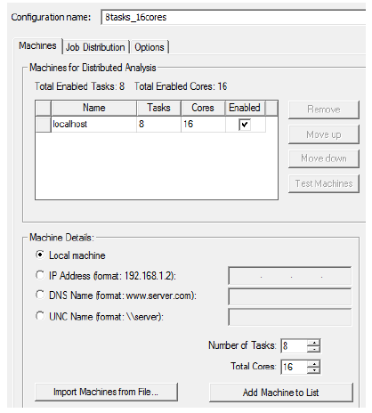
HPC analysis and configuration options

For example in figure above, 16 cores are available on the machine in which the design was simulated. In a set up of 8 tasks executed with these 16 cores, the sweep is run with 8 frequency points being solved in parallel using two cores of matrix multiprocessing for each frequency point. When such an analysis is executed on a single machine, the simulation is very efficient if the machine has enough shared memory to accommodate 8 simultaneous solves. Otherwise the analysis could be performed across multiple machines (that have HFSS installed in them) without requiring any additional HFSS license for each machine.

The advantage of deembedding is that it saves the trouble of explicitly modeling the long cable lengths. Such a design is efficient and can be solved using minimum computational resources. By using HPC, the solution time is further reduced.

Results

The following figure shows the S-parameter plot.

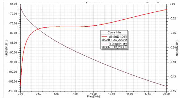
s-parameter plot